

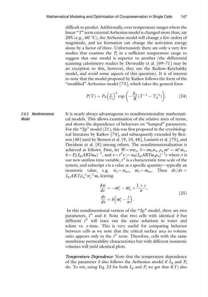
difficult to predict. Additionally, over temperature ranges where the
linear “T” term external Arrhenius model is changed more than, say
20% (e.g., 60
∘
C), the Arrhenius model will change a few orders of
magnitude, and ice formation can change the activation energy
alone by a factor of three. Unfortunately there are only a very few
studies that examine the P s in a sufficient temperature range to
suggest that one model is superior to another (the differential
scanning calorimetry studies by Devireddy et al. [69–71] may be
an exception to this, however, they use the Kedem–Ketchalsky
model, and avoid some aspects of this question). It is of interest
to note that the model proposed by Katkov follows the form of the
“modified” Arrhenius model [73], which takes the general form
PðT Þ ¼ P 0
T
T 0
n
exp À
E a
R
ðT
À1
À T
À1
0 Þ
:
ð24Þ
2.4.3 Nondimensional
Model
It is nearly always advantageous to nondimensionalize mathematical models. This allows examination of the relative sizes of terms,
and shows the dependence of behaviors on “lumped” parameters.
For the “2p” model (21), this was first proposed in the cryobiological literature by Katkov [74], and subsequently extended by Benson [48] used by Benson et al. [9, 10, 48], Lusianti et al. [75], and
Davidson et al. [8] among others. The nondimensionalization is
achieved as follows. First, let W ¼ ww o , S ¼ sm o w o , ρ w m
e
Á ¼
m
e
Á m o ,
b ¼ P s (L p ARTm 0 )
À1 , and t ¼ t
∗
τ :¼ w 0 (L p ARTm o ρ w )
À1
τ where τ is
our new unitless time variable, t
∗ is a characteristic time scale of the
system, and subscript o is a value at a specific quantity—typically an
isosmotic value, e.g. w o ¼ w iso , m o ¼ m iso . Then dt=dτ ¼
L p ART ρ
À1
w w
À1
o m o leaving
dw
dτ
¼ À
m
e
s À
m
e
n þ
1 þ s
w
,
ds
dτ
¼ b
m
e
s À
s
w
:
ð25Þ
In this nondimensional version of the “2p” model, there are two
parameters, t
∗ and b. Note that two cells with identical b but
different t
∗ will trace out the same solutions in water and
solute vs. τ-time. This is very useful for comparing behavior
between cells as we note that the critical surface area to volume
ratio appears only in the t
∗ term. Therefore, cells with the same
membrane permeability characteristics but with different isosmotic
volumes will yield identical plots.
Temperature Dependence: Note that the temperature dependence
of the parameter b also follows the Arrhenius model if L p and P s
do. To wit, using Eq. 23 for both L p and P s we get that b(T) also
Mathematical Modeling and Optimization of Cryopreservation in Single Cells
147
linear “T” term external Arrhenius model is changed more than, say
20% (e.g., 60
∘
C), the Arrhenius model will change a few orders of
magnitude, and ice formation can change the activation energy
alone by a factor of three. Unfortunately there are only a very few
studies that examine the P s in a sufficient temperature range to
suggest that one model is superior to another (the differential
scanning calorimetry studies by Devireddy et al. [69–71] may be
an exception to this, however, they use the Kedem–Ketchalsky
model, and avoid some aspects of this question). It is of interest
to note that the model proposed by Katkov follows the form of the
“modified” Arrhenius model [73], which takes the general form
PðT Þ ¼ P 0
T
T 0
n
exp À
E a
R
ðT
À1
À T
À1
0 Þ
:
ð24Þ
2.4.3 Nondimensional
Model
It is nearly always advantageous to nondimensionalize mathematical models. This allows examination of the relative sizes of terms,
and shows the dependence of behaviors on “lumped” parameters.
For the “2p” model (21), this was first proposed in the cryobiological literature by Katkov [74], and subsequently extended by Benson [48] used by Benson et al. [9, 10, 48], Lusianti et al. [75], and
Davidson et al. [8] among others. The nondimensionalization is
achieved as follows. First, let W ¼ ww o , S ¼ sm o w o , ρ w m
e
Á ¼
m
e
Á m o ,
b ¼ P s (L p ARTm 0 )
À1 , and t ¼ t
∗
τ :¼ w 0 (L p ARTm o ρ w )
À1
τ where τ is
our new unitless time variable, t
∗ is a characteristic time scale of the
system, and subscript o is a value at a specific quantity—typically an
isosmotic value, e.g. w o ¼ w iso , m o ¼ m iso . Then dt=dτ ¼
L p ART ρ
À1
w w
À1
o m o leaving
dw
dτ
¼ À
m
e
s À
m
e
n þ
1 þ s
w
,
ds
dτ
¼ b
m
e
s À
s
w
:
ð25Þ
In this nondimensional version of the “2p” model, there are two
parameters, t
∗ and b. Note that two cells with identical b but
different t
∗ will trace out the same solutions in water and
solute vs. τ-time. This is very useful for comparing behavior
between cells as we note that the critical surface area to volume
ratio appears only in the t
∗ term. Therefore, cells with the same
membrane permeability characteristics but with different isosmotic
volumes will yield identical plots.
Temperature Dependence: Note that the temperature dependence
of the parameter b also follows the Arrhenius model if L p and P s
do. To wit, using Eq. 23 for both L p and P s we get that b(T) also
Mathematical Modeling and Optimization of Cryopreservation in Single Cells
147