

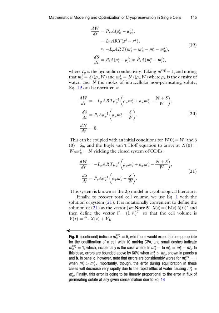
dW
dt
¼ P w Aðμ
e
w À μ
i
w Þ,
¼ L p ART ðπ
i
À π
e
Þ,
% ÀL p ART ðm
e
s þ m
e
n À m
i
s À m
i
n Þ,
dS
dt
¼ P s Aðμ
e
s À μ
i
s Þ % ~
P s Aðm
e
s À m
i
s Þ,
ð19Þ
where L p is the hydraulic conductivity. Taking m
avg
¼ 1, and noting
that m
i
s ¼ S=ðρ w W Þ and m
i
n ¼ N =ðρ w W Þ where ρ w is the density of
water, and N the moles of intracellular non-permeating solute,
Eq. 19 can be rewritten as
dW
dt
¼ ÀL p ART ρ
À1
w
ρ w m
e
s þ ρ w m
e
n À
N þ S
W
,
dS
dt
¼ P s Aρ
À1
w
ρ w m
e
s À
S
W
,
dN
dt
¼ 0:
ð20Þ
This can be coupled with an initial conditions for W(0) ¼ W 0 and S
(0) ¼ S 0 , and the Boyle van ’t Hoff equation to arrive at N ð0Þ ¼
W 0 m
i
n ¼ N yielding the closed system of ODEs:
dW
dt
¼ ÀL p ART ρ
À1
w
ρ w m
e
s þ ρ w m
e
n À
N þ S
W
,
dS
dt
¼ P s Aρ
À1
w
ρ w m
e
s À
S
W
:
ð21Þ
This system is known as the 2p model in cryobiological literature.
Finally, to recover total cell volume, we use Eq. 1 with the
solution of system (21). It is notationally convenient to define the
solution of (21) as the vector (see Note 5) X(t) ¼ (W(t) S(t))
T and
then define the vector
Γ ¼ ð1
v s Þ
T so that the cell volume is
V ðtÞ ¼
Γ Á X ðtÞ þ V b .
ä
Fig. 5 (continued) indicate m
avg
s ¼ 5, which one would expect to be appropriate
for the equilibration of a cell with 10 mol/kg CPA, and small dashes indicate
m
avg
s ¼ 1, which, incidentally is the case where ln m
e
s À ln m
i
s % m
e
s À m
i
s . In
this case, errors are bounded above by 60% when m
e
s > m
i
s , shown in panels a
and b. In panel c, however, note that errors are considerably worse for m
avg
s ¼ 1
when m
i
s > m
e
s . Importantly, though, the error during equilibration in these
cases will decrease very rapidly due to the rapid efflux of water causing m
e
s %
m
i
s . Finally, this error is going to be linearly proportional to the error in flux of
permeating solute at any given concentration due to Eq. 14
Mathematical Modeling and Optimization of Cryopreservation in Single Cells
145
dt
¼ P w Aðμ
e
w À μ
i
w Þ,
¼ L p ART ðπ
i
À π
e
Þ,
% ÀL p ART ðm
e
s þ m
e
n À m
i
s À m
i
n Þ,
dS
dt
¼ P s Aðμ
e
s À μ
i
s Þ % ~
P s Aðm
e
s À m
i
s Þ,
ð19Þ
where L p is the hydraulic conductivity. Taking m
avg
¼ 1, and noting
that m
i
s ¼ S=ðρ w W Þ and m
i
n ¼ N =ðρ w W Þ where ρ w is the density of
water, and N the moles of intracellular non-permeating solute,
Eq. 19 can be rewritten as
dW
dt
¼ ÀL p ART ρ
À1
w
ρ w m
e
s þ ρ w m
e
n À
N þ S
W
,
dS
dt
¼ P s Aρ
À1
w
ρ w m
e
s À
S
W
,
dN
dt
¼ 0:
ð20Þ
This can be coupled with an initial conditions for W(0) ¼ W 0 and S
(0) ¼ S 0 , and the Boyle van ’t Hoff equation to arrive at N ð0Þ ¼
W 0 m
i
n ¼ N yielding the closed system of ODEs:
dW
dt
¼ ÀL p ART ρ
À1
w
ρ w m
e
s þ ρ w m
e
n À
N þ S
W
,
dS
dt
¼ P s Aρ
À1
w
ρ w m
e
s À
S
W
:
ð21Þ
This system is known as the 2p model in cryobiological literature.
Finally, to recover total cell volume, we use Eq. 1 with the
solution of system (21). It is notationally convenient to define the
solution of (21) as the vector (see Note 5) X(t) ¼ (W(t) S(t))
T and
then define the vector
Γ ¼ ð1
v s Þ
T so that the cell volume is
V ðtÞ ¼
Γ Á X ðtÞ þ V b .
ä
Fig. 5 (continued) indicate m
avg
s ¼ 5, which one would expect to be appropriate
for the equilibration of a cell with 10 mol/kg CPA, and small dashes indicate
m
avg
s ¼ 1, which, incidentally is the case where ln m
e
s À ln m
i
s % m
e
s À m
i
s . In
this case, errors are bounded above by 60% when m
e
s > m
i
s , shown in panels a
and b. In panel c, however, note that errors are considerably worse for m
avg
s ¼ 1
when m
i
s > m
e
s . Importantly, though, the error during equilibration in these
cases will decrease very rapidly due to the rapid efflux of water causing m
e
s %
m
i
s . Finally, this error is going to be linearly proportional to the error in flux of
permeating solute at any given concentration due to Eq. 14
Mathematical Modeling and Optimization of Cryopreservation in Single Cells
145