

for details]. Using the same formalism and mixing rules defined for
the osmotic virial Eq. 9, the chemical potential of the ith solute as a
function of m ¼ (m 1 , . . ., m n )
T is
μ i ðmÞ ¼ RT ln m i þ Ψ
∗
i þ
P n
j ¼1
ðB i þ B j Þm j
!
,
ð13Þ
where Ψ
∗
i is a function of temperature and pressure, and B i are
defined above.
2.4 Membrane
Transport Models
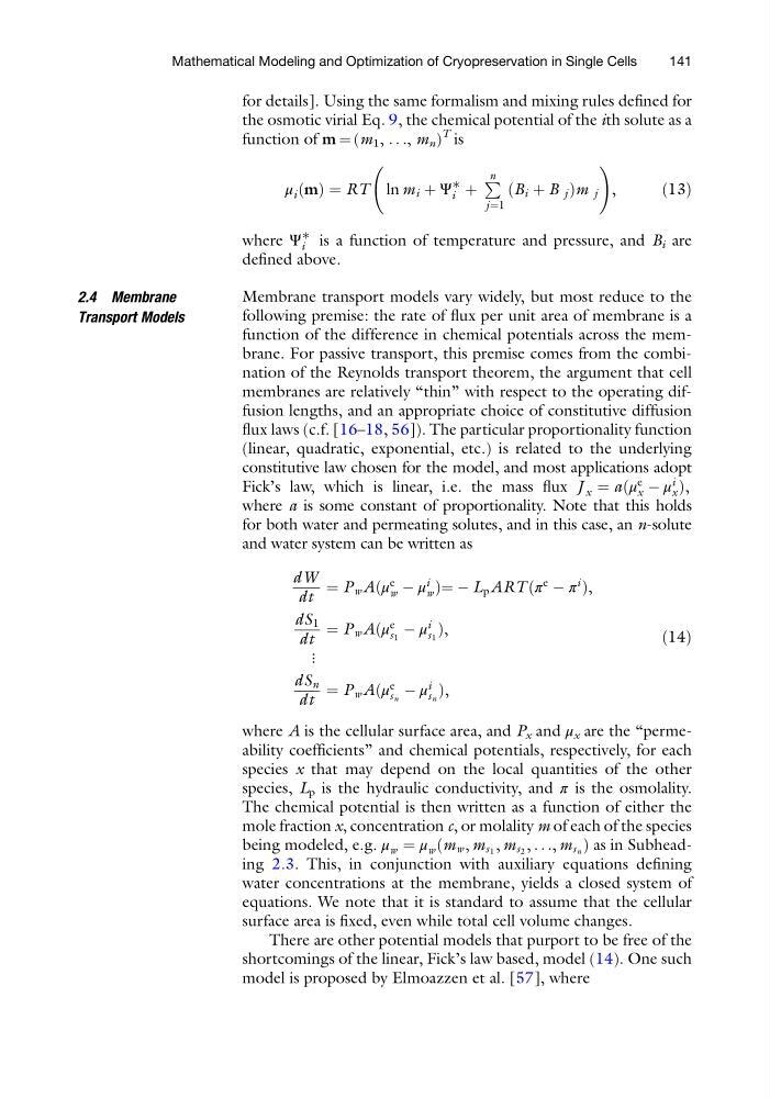
Membrane transport models vary widely, but most reduce to the
following premise: the rate of flux per unit area of membrane is a
function of the difference in chemical potentials across the membrane. For passive transport, this premise comes from the combination of the Reynolds transport theorem, the argument that cell
membranes are relatively “thin” with respect to the operating diffusion lengths, and an appropriate choice of constitutive diffusion
flux laws (c.f. [16–18, 56]). The particular proportionality function
(linear, quadratic, exponential, etc.) is related to the underlying
constitutive law chosen for the model, and most applications adopt
Fick’s law, which is linear, i.e. the mass flux J x ¼ aðμ
e
x À μ
i
x Þ,
where a is some constant of proportionality. Note that this holds
for both water and permeating solutes, and in this case, an n-solute
and water system can be written as
dW
dt
¼ P w Aðμ
e
w À μ
i
w Þ¼ À L p ART ðπ
e
À π
i
Þ,
dS 1
dt
¼ P w Aðμ
e
s 1
À μ
i
s 1
Þ,
⋮
dS n
dt
¼ P w Aðμ
e
s n
À μ
i
s n
Þ,
ð14Þ
where A is the cellular surface area, and P x and μ x are the “permeability coefficients” and chemical potentials, respectively, for each
species x that may depend on the local quantities of the other
species, L p is the hydraulic conductivity, and π is the osmolality.
The chemical potential is then written as a function of either the
mole fraction x, concentration c, or molality m of each of the species
being modeled, e.g. μ w ¼ μ w ðm w , m s 1 , m s 2 , . . ., m s n Þ as in Subheading 2.3. This, in conjunction with auxiliary equations defining
water concentrations at the membrane, yields a closed system of
equations. We note that it is standard to assume that the cellular
surface area is fixed, even while total cell volume changes.
There are other potential models that purport to be free of the
shortcomings of the linear, Fick’s law based, model (14). One such
model is proposed by Elmoazzen et al. [57], where
Mathematical Modeling and Optimization of Cryopreservation in Single Cells
141
the osmotic virial Eq. 9, the chemical potential of the ith solute as a
function of m ¼ (m 1 , . . ., m n )
T is
μ i ðmÞ ¼ RT ln m i þ Ψ
∗
i þ
P n
j ¼1
ðB i þ B j Þm j
!
,
ð13Þ
where Ψ
∗
i is a function of temperature and pressure, and B i are
defined above.
2.4 Membrane
Transport Models
Membrane transport models vary widely, but most reduce to the
following premise: the rate of flux per unit area of membrane is a
function of the difference in chemical potentials across the membrane. For passive transport, this premise comes from the combination of the Reynolds transport theorem, the argument that cell
membranes are relatively “thin” with respect to the operating diffusion lengths, and an appropriate choice of constitutive diffusion
flux laws (c.f. [16–18, 56]). The particular proportionality function
(linear, quadratic, exponential, etc.) is related to the underlying
constitutive law chosen for the model, and most applications adopt
Fick’s law, which is linear, i.e. the mass flux J x ¼ aðμ
e
x À μ
i
x Þ,
where a is some constant of proportionality. Note that this holds
for both water and permeating solutes, and in this case, an n-solute
and water system can be written as
dW
dt
¼ P w Aðμ
e
w À μ
i
w Þ¼ À L p ART ðπ
e
À π
i
Þ,
dS 1
dt
¼ P w Aðμ
e
s 1
À μ
i
s 1
Þ,
⋮
dS n
dt
¼ P w Aðμ
e
s n
À μ
i
s n
Þ,
ð14Þ
where A is the cellular surface area, and P x and μ x are the “permeability coefficients” and chemical potentials, respectively, for each
species x that may depend on the local quantities of the other
species, L p is the hydraulic conductivity, and π is the osmolality.
The chemical potential is then written as a function of either the
mole fraction x, concentration c, or molality m of each of the species
being modeled, e.g. μ w ¼ μ w ðm w , m s 1 , m s 2 , . . ., m s n Þ as in Subheading 2.3. This, in conjunction with auxiliary equations defining
water concentrations at the membrane, yields a closed system of
equations. We note that it is standard to assume that the cellular
surface area is fixed, even while total cell volume changes.
There are other potential models that purport to be free of the
shortcomings of the linear, Fick’s law based, model (14). One such
model is proposed by Elmoazzen et al. [57], where
Mathematical Modeling and Optimization of Cryopreservation in Single Cells
141