

m 1 ¼ Rm 2 ,
m 2 ¼
ffiffiffiffiffiffiffiffiffiffiffiffiffiffiffiffiffiffiffiffiffiffiffiffiffiffiffiffiffiffiffiffiffiffiffiffiffiffiffiffiffiffiffiffiffiffiffiffiffiffiffiffiffiffiffiffiffiffiffiffiffiffiffiffiffiffiffiffiffiffiffiffiffiffiffiffiffiffiffiffiffiffiffiffiffiffiffiffiffiffiffiffiffiffiffiffiffiffiffi ffi
1 þ 4B 2 θ þ R
2
ð1 þ 4B 1 θÞ þ 2Rð1 þ B 1 θ þ B 2 θÞ
q
À 1 À R
B 2 ð2 þ RÞ þ B 1 Rð1 þ 2RÞ
:
ð12Þ
2.3.2 Chemical Potential
Osmolality models facilitate the prediction of the melting temperature and the likelihood that water will crystalize. It is useful to
derive the concentrations or molalities of the constituent solutes.
However, water and solute transport is driven by chemical potential
gradients. In the case of water transport, note that μ w ¼ μ
0
w À RT π,
where μ
0
w is the chemical potential of pure water at standard temperature and pressure. Thus osmolality is sufficient for modeling
water transport. For solute transport, however, other models must
be used. The most common approximation for chemical potential is
that μ s ðm s Þ % RT ln m s , but one may arrive at a more accurate form
by starting with the same “virial” energy used to derive model (9),
and differentiating with respect to the moles of solute [see ref. 55,
0.1
0.2
0.3
0.4
0.5
0
10
20
30
40
Total mass fraction
Freezing Point Depression (ºC)
Fit Model
Quadratic Virial
Cubic Virial
Additive Model
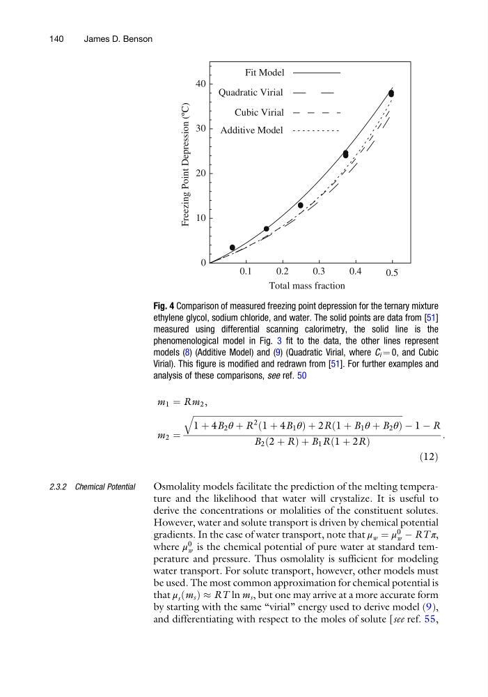
Fig. 4 Comparison of measured freezing point depression for the ternary mixture
ethylene glycol, sodium chloride, and water. The solid points are data from [51]
measured using differential scanning calorimetry, the solid line is the
phenomenological model in Fig. 3 fit to the data, the other lines represent
models (8) (Additive Model) and (9) (Quadratic Virial, where C i ¼ 0, and Cubic
Virial). This figure is modified and redrawn from [51]. For further examples and
analysis of these comparisons, see ref. 50
140
James D. Benson
m 2 ¼
ffiffiffiffiffiffiffiffiffiffiffiffiffiffiffiffiffiffiffiffiffiffiffiffiffiffiffiffiffiffiffiffiffiffiffiffiffiffiffiffiffiffiffiffiffiffiffiffiffiffiffiffiffiffiffiffiffiffiffiffiffiffiffiffiffiffiffiffiffiffiffiffiffiffiffiffiffiffiffiffiffiffiffiffiffiffiffiffiffiffiffiffiffiffiffiffiffiffiffi ffi
1 þ 4B 2 θ þ R
2
ð1 þ 4B 1 θÞ þ 2Rð1 þ B 1 θ þ B 2 θÞ
q
À 1 À R
B 2 ð2 þ RÞ þ B 1 Rð1 þ 2RÞ
:
ð12Þ
2.3.2 Chemical Potential
Osmolality models facilitate the prediction of the melting temperature and the likelihood that water will crystalize. It is useful to
derive the concentrations or molalities of the constituent solutes.
However, water and solute transport is driven by chemical potential
gradients. In the case of water transport, note that μ w ¼ μ
0
w À RT π,
where μ
0
w is the chemical potential of pure water at standard temperature and pressure. Thus osmolality is sufficient for modeling
water transport. For solute transport, however, other models must
be used. The most common approximation for chemical potential is
that μ s ðm s Þ % RT ln m s , but one may arrive at a more accurate form
by starting with the same “virial” energy used to derive model (9),
and differentiating with respect to the moles of solute [see ref. 55,
0.1
0.2
0.3
0.4
0.5
0
10
20
30
40
Total mass fraction
Freezing Point Depression (ºC)
Fit Model
Quadratic Virial
Cubic Virial
Additive Model
Fig. 4 Comparison of measured freezing point depression for the ternary mixture
ethylene glycol, sodium chloride, and water. The solid points are data from [51]
measured using differential scanning calorimetry, the solid line is the
phenomenological model in Fig. 3 fit to the data, the other lines represent
models (8) (Additive Model) and (9) (Quadratic Virial, where C i ¼ 0, and Cubic
Virial). This figure is modified and redrawn from [51]. For further examples and
analysis of these comparisons, see ref. 50
140
James D. Benson