

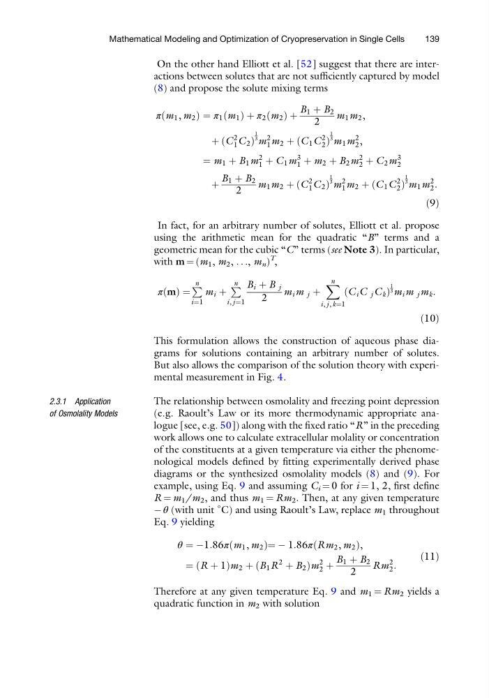
On the other hand Elliott et al. [52] suggest that there are interactions between solutes that are not sufficiently captured by model
(8) and propose the solute mixing terms
πðm 1 , m 2 Þ ¼ π 1 ðm 1 Þ þ π 2 ðm 2 Þ þ
B 1 þ B 2
2
m 1 m 2 ,
þ ðC
2
1 C 2 Þ
1
3 m
2
1 m 2 þ ðC 1 C
2
2 Þ
1
3 m 1 m
2
2 ,
¼ m 1 þ B 1 m
2
1 þ C 1 m
3
1 þ m 2 þ B 2 m
2
2 þ C 2 m
3
2
þ
B 1 þ B 2
2
m 1 m 2 þ ðC
2
1 C 2 Þ
1
3 m
2
1 m 2 þ ðC 1 C
2
2 Þ
1
3 m 1 m
2
2 :
ð9Þ
In fact, for an arbitrary number of solutes, Elliott et al. propose
using the arithmetic mean for the quadratic “B” terms and a
geometric mean for the cubic “C” terms (see Note 3). In particular,
with m ¼ (m 1 , m 2 , . . ., m n )
T
,
πðmÞ ¼
P n
i¼1
m i þ
P n
i, j ¼1
B i þ B j
2
m i m j þ
X n
i, j , k¼1
ðC i C j C k Þ
1
3 m i m j m k :
ð10Þ
This formulation allows the construction of aqueous phase diagrams for solutions containing an arbitrary number of solutes.
But also allows the comparison of the solution theory with experimental measurement in Fig. 4.
2.3.1 Application
of Osmolality Models
The relationship between osmolality and freezing point depression
(e.g. Raoult’s Law or its more thermodynamic appropriate analogue [see, e.g. 50]) along with the fixed ratio “R” in the preceding
work allows one to calculate extracellular molality or concentration
of the constituents at a given temperature via either the phenomenological models defined by fitting experimentally derived phase
diagrams or the synthesized osmolality models (8) and (9). For
example, using Eq. 9 and assuming C i ¼ 0 for i ¼ 1, 2, first define
R ¼ m 1 /m 2 , and thus m 1 ¼ Rm 2 . Then, at any given temperature
À θ (with unit
∘
C) and using Raoult’s Law, replace m 1 throughout
Eq. 9 yielding
θ ¼ À1:86πðm 1 , m 2 Þ¼ À 1:86πðRm 2 , m 2 Þ,
¼ ðR þ 1Þm 2 þ ðB 1 R
2
þ B 2 Þm
2
2 þ
B 1 þ B 2
2
Rm
2
2 :
ð11Þ
Therefore at any given temperature Eq. 9 and m 1 ¼ Rm 2 yields a
quadratic function in m 2 with solution
Mathematical Modeling and Optimization of Cryopreservation in Single Cells
139
(8) and propose the solute mixing terms
πðm 1 , m 2 Þ ¼ π 1 ðm 1 Þ þ π 2 ðm 2 Þ þ
B 1 þ B 2
2
m 1 m 2 ,
þ ðC
2
1 C 2 Þ
1
3 m
2
1 m 2 þ ðC 1 C
2
2 Þ
1
3 m 1 m
2
2 ,
¼ m 1 þ B 1 m
2
1 þ C 1 m
3
1 þ m 2 þ B 2 m
2
2 þ C 2 m
3
2
þ
B 1 þ B 2
2
m 1 m 2 þ ðC
2
1 C 2 Þ
1
3 m
2
1 m 2 þ ðC 1 C
2
2 Þ
1
3 m 1 m
2
2 :
ð9Þ
In fact, for an arbitrary number of solutes, Elliott et al. propose
using the arithmetic mean for the quadratic “B” terms and a
geometric mean for the cubic “C” terms (see Note 3). In particular,
with m ¼ (m 1 , m 2 , . . ., m n )
T
,
πðmÞ ¼
P n
i¼1
m i þ
P n
i, j ¼1
B i þ B j
2
m i m j þ
X n
i, j , k¼1
ðC i C j C k Þ
1
3 m i m j m k :
ð10Þ
This formulation allows the construction of aqueous phase diagrams for solutions containing an arbitrary number of solutes.
But also allows the comparison of the solution theory with experimental measurement in Fig. 4.
2.3.1 Application
of Osmolality Models
The relationship between osmolality and freezing point depression
(e.g. Raoult’s Law or its more thermodynamic appropriate analogue [see, e.g. 50]) along with the fixed ratio “R” in the preceding
work allows one to calculate extracellular molality or concentration
of the constituents at a given temperature via either the phenomenological models defined by fitting experimentally derived phase
diagrams or the synthesized osmolality models (8) and (9). For
example, using Eq. 9 and assuming C i ¼ 0 for i ¼ 1, 2, first define
R ¼ m 1 /m 2 , and thus m 1 ¼ Rm 2 . Then, at any given temperature
À θ (with unit
∘
C) and using Raoult’s Law, replace m 1 throughout
Eq. 9 yielding
θ ¼ À1:86πðm 1 , m 2 Þ¼ À 1:86πðRm 2 , m 2 Þ,
¼ ðR þ 1Þm 2 þ ðB 1 R
2
þ B 2 Þm
2
2 þ
B 1 þ B 2
2
Rm
2
2 :
ð11Þ
Therefore at any given temperature Eq. 9 and m 1 ¼ Rm 2 yields a
quadratic function in m 2 with solution
Mathematical Modeling and Optimization of Cryopreservation in Single Cells
139