

2.1 Maxwell’s Equations in the Presence of Water
53
where the frequency-dependent function is the dielectric function of the
medium, which is a function of its thermodynamic state and obeys the dispersion law:
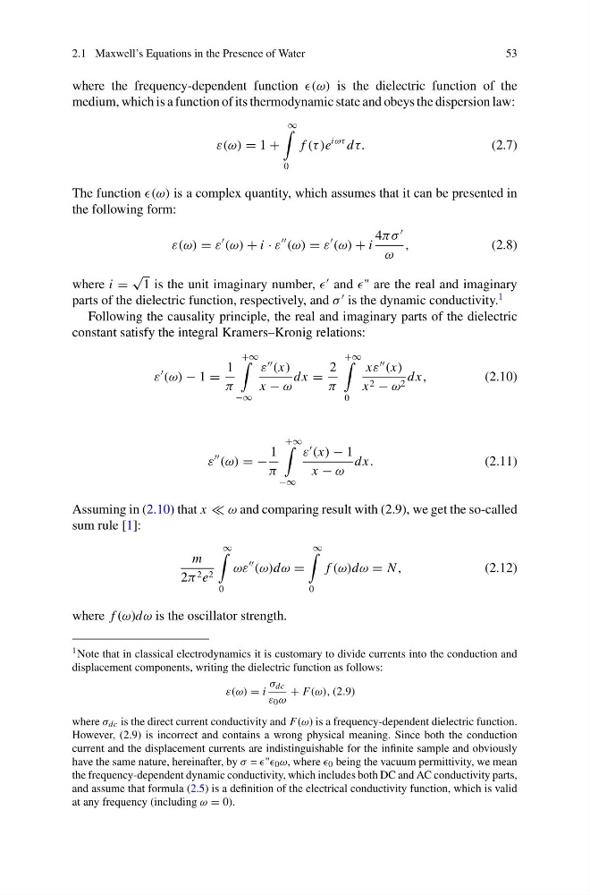
ε(ω) = 1 +
∞
0
f (τ )e
iωτ dτ.
(2.7)
The function is a complex quantity, which assumes that it can be presented in
the following form:
ε(ω) = ε
(ω) + i · ε
(ω) = ε
(ω) + i
4πσ
ω
,
(2.8)
where i =
√
1 is the unit imaginary number,
and " are the real and imaginary
parts of the dielectric function, respectively, and σ
is the dynamic conductivity.
1
Following the causality principle, the real and imaginary parts of the dielectric
constant satisfy the integral Kramers–Kronig relations:
ε
(ω) − 1 =
1
π
+∞
−∞
ε
(x)
x − ω
dx =
2
π
+∞
0
xε
(x)
x 2 − ω 2 dx,
(2.10)
ε
(ω) = −
1
π
+∞
−∞
ε
(x) − 1
x − ω
dx.
(2.11)
Assuming in (2.10) that x ω and comparing result with (2.9), we get the so-called
sum rule [1]:
m
2π 2 e 2
∞
0
ωε
(ω)dω =
∞
0
f (ω)dω = N ,
(2.12)
where f (ω)dω is the oscillator strength.
1 Note that in classical electrodynamics it is customary to divide currents into the conduction and
displacement components, writing the dielectric function as follows:
ε(ω) = i
σ dc
ε 0 ω
+ F(ω), (2.9)
where σ dc is the direct current conductivity and F(ω) is a frequency-dependent dielectric function.
However, (2.9) is incorrect and contains a wrong physical meaning. Since both the conduction
current and the displacement currents are indistinguishable for the infinite sample and obviously
have the same nature, hereinafter, by σ = " 0 ω, where 0 being the vacuum permittivity, we mean
the frequency-dependent dynamic conductivity, which includes both DC and AC conductivity parts,
and assume that formula (2.5) is a definition of the electrical conductivity function, which is valid
at any frequency (including ω = 0).
53
where the frequency-dependent function is the dielectric function of the
medium, which is a function of its thermodynamic state and obeys the dispersion law:
ε(ω) = 1 +
∞
0
f (τ )e
iωτ dτ.
(2.7)
The function is a complex quantity, which assumes that it can be presented in
the following form:
ε(ω) = ε
(ω) + i · ε
(ω) = ε
(ω) + i
4πσ
ω
,
(2.8)
where i =
√
1 is the unit imaginary number,
and " are the real and imaginary
parts of the dielectric function, respectively, and σ
is the dynamic conductivity.
1
Following the causality principle, the real and imaginary parts of the dielectric
constant satisfy the integral Kramers–Kronig relations:
ε
(ω) − 1 =
1
π
+∞
−∞
ε
(x)
x − ω
dx =
2
π
+∞
0
xε
(x)
x 2 − ω 2 dx,
(2.10)
ε
(ω) = −
1
π
+∞
−∞
ε
(x) − 1
x − ω
dx.
(2.11)
Assuming in (2.10) that x ω and comparing result with (2.9), we get the so-called
sum rule [1]:
m
2π 2 e 2
∞
0
ωε
(ω)dω =
∞
0
f (ω)dω = N ,
(2.12)
where f (ω)dω is the oscillator strength.
1 Note that in classical electrodynamics it is customary to divide currents into the conduction and
displacement components, writing the dielectric function as follows:
ε(ω) = i
σ dc
ε 0 ω
+ F(ω), (2.9)
where σ dc is the direct current conductivity and F(ω) is a frequency-dependent dielectric function.
However, (2.9) is incorrect and contains a wrong physical meaning. Since both the conduction
current and the displacement currents are indistinguishable for the infinite sample and obviously
have the same nature, hereinafter, by σ = " 0 ω, where 0 being the vacuum permittivity, we mean
the frequency-dependent dynamic conductivity, which includes both DC and AC conductivity parts,
and assume that formula (2.5) is a definition of the electrical conductivity function, which is valid
at any frequency (including ω = 0).