

52
2 The Interaction of Electromagnetic Waves with Water
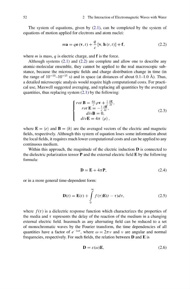
The system of equations, given by (2.1), can be completed by the system of
equations of motion applied for electrons and atom nuclei:
ma = qe (v, t) +
q
c
[v, h (r, t)] + f,
(2.2)
where m is mass, q is electric charge, and f is the force.
Although systems (2.1) and (2.2) are complete and allow one to describe any
atomic-molecular ensemble, they cannot be applied to the real macroscopic substance, because the microscopic fields and charge distribution change in time (in
the range of 10
−10 –10
−15 s) and in space (at distances of about 0.1–1.0 Å). Thus,
a detailed microscopic analysis would require high computational costs. For practical use, Maxwell suggested averaging, and replacing all quantities by the averaged
quantities, thus replacing system (2.1) by the following:
⎧
⎪ ⎪ ⎨
⎪ ⎪ ⎩
rot B =
4π
c
ρv +
1
c
∂E
∂t
,
rot E = −
1
c
∂B
∂t
,
divB = 0,
divE = 4π ρ ,
(2.3)
where E = =e and B = =h are the averaged vectors of the electric and magnetic
fields, respectively. Although this system of equation loses some information about
the local fields, it requires much lower computational costs and can be applied to any
continuous medium.
Within this approach, the magnitude of the electric induction D is connected to
the dielectric polarization tensor P and the external electric field E by the following
formula:
D = E + 4π P,
(2.4)
or in a more general time-dependent form:
D(t) = E(t) +
∞
0
f (τ )E(t − τ )dτ,
(2.5)
where f (τ ) is a dielectric response function which characterizes the properties of
the media and τ represents the delay of the reaction of the medium in a changing
external electric field. Inasmuch as any alternating field can be reduced to a set
of monochromatic waves by the Fourier transform, the time dependencies of all
quantities have a factor of e
−iωt , where ω = 2πν and ν are angular and normal
frequencies, respectively. For such fields, the relation between D and E is
D = ε(ω)E,
(2.6)
2 The Interaction of Electromagnetic Waves with Water
The system of equations, given by (2.1), can be completed by the system of
equations of motion applied for electrons and atom nuclei:
ma = qe (v, t) +
q
c
[v, h (r, t)] + f,
(2.2)
where m is mass, q is electric charge, and f is the force.
Although systems (2.1) and (2.2) are complete and allow one to describe any
atomic-molecular ensemble, they cannot be applied to the real macroscopic substance, because the microscopic fields and charge distribution change in time (in
the range of 10
−10 –10
−15 s) and in space (at distances of about 0.1–1.0 Å). Thus,
a detailed microscopic analysis would require high computational costs. For practical use, Maxwell suggested averaging, and replacing all quantities by the averaged
quantities, thus replacing system (2.1) by the following:
⎧
⎪ ⎪ ⎨
⎪ ⎪ ⎩
rot B =
4π
c
ρv +
1
c
∂E
∂t
,
rot E = −
1
c
∂B
∂t
,
divB = 0,
divE = 4π ρ ,
(2.3)
where E = =e and B = =h are the averaged vectors of the electric and magnetic
fields, respectively. Although this system of equation loses some information about
the local fields, it requires much lower computational costs and can be applied to any
continuous medium.
Within this approach, the magnitude of the electric induction D is connected to
the dielectric polarization tensor P and the external electric field E by the following
formula:
D = E + 4π P,
(2.4)
or in a more general time-dependent form:
D(t) = E(t) +
∞
0
f (τ )E(t − τ )dτ,
(2.5)
where f (τ ) is a dielectric response function which characterizes the properties of
the media and τ represents the delay of the reaction of the medium in a changing
external electric field. Inasmuch as any alternating field can be reduced to a set
of monochromatic waves by the Fourier transform, the time dependencies of all
quantities have a factor of e
−iωt , where ω = 2πν and ν are angular and normal
frequencies, respectively. For such fields, the relation between D and E is
D = ε(ω)E,
(2.6)