

1.2 Bragg Scattering and Bernal–Fowler Water
11
H
O
H
O
H
O
H
O
H O
H
O
H
O
H O
H
O
H
O
H
O
H
O
p
+
(a)
(b)
H
H
H
H
H
H
H
H
H
H
H
H
2
1
2
2
2
2
2
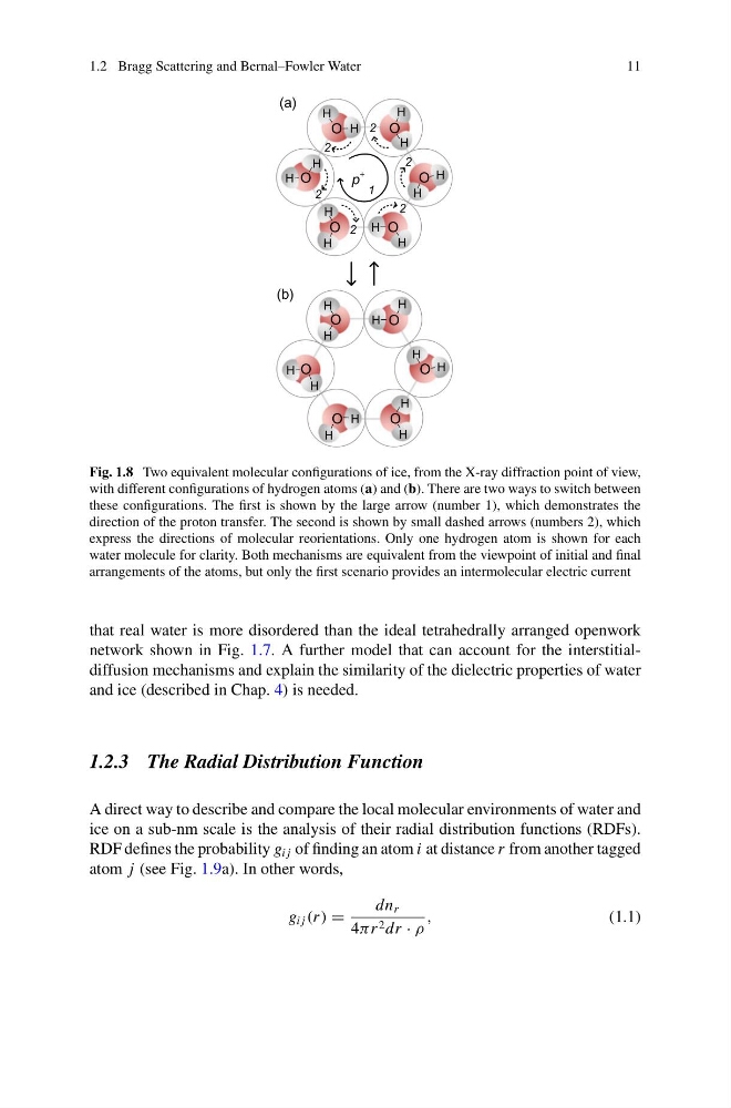
Fig. 1.8 Two equivalent molecular configurations of ice, from the X-ray diffraction point of view,
with different configurations of hydrogen atoms (a) and (b). There are two ways to switch between
these configurations. The first is shown by the large arrow (number 1), which demonstrates the
direction of the proton transfer. The second is shown by small dashed arrows (numbers 2), which
express the directions of molecular reorientations. Only one hydrogen atom is shown for each
water molecule for clarity. Both mechanisms are equivalent from the viewpoint of initial and final
arrangements of the atoms, but only the first scenario provides an intermolecular electric current
that real water is more disordered than the ideal tetrahedrally arranged openwork
network shown in Fig. 1.7. A further model that can account for the interstitialdiffusion mechanisms and explain the similarity of the dielectric properties of water
and ice (described in Chap. 4) is needed.
1.2.3 The Radial Distribution Function
A direct way to describe and compare the local molecular environments of water and
ice on a sub-nm scale is the analysis of their radial distribution functions (RDFs).
RDF defines the probability g i j of finding an atom i at distance r from another tagged
atom j (see Fig. 1.9a). In other words,
g i j (r ) =
dn r
4πr 2 dr · ρ
,
(1.1)
11
H
O
H
O
H
O
H
O
H O
H
O
H
O
H O
H
O
H
O
H
O
H
O
p
+
(a)
(b)
H
H
H
H
H
H
H
H
H
H
H
H
2
1
2
2
2
2
2
Fig. 1.8 Two equivalent molecular configurations of ice, from the X-ray diffraction point of view,
with different configurations of hydrogen atoms (a) and (b). There are two ways to switch between
these configurations. The first is shown by the large arrow (number 1), which demonstrates the
direction of the proton transfer. The second is shown by small dashed arrows (numbers 2), which
express the directions of molecular reorientations. Only one hydrogen atom is shown for each
water molecule for clarity. Both mechanisms are equivalent from the viewpoint of initial and final
arrangements of the atoms, but only the first scenario provides an intermolecular electric current
that real water is more disordered than the ideal tetrahedrally arranged openwork
network shown in Fig. 1.7. A further model that can account for the interstitialdiffusion mechanisms and explain the similarity of the dielectric properties of water
and ice (described in Chap. 4) is needed.
1.2.3 The Radial Distribution Function
A direct way to describe and compare the local molecular environments of water and
ice on a sub-nm scale is the analysis of their radial distribution functions (RDFs).
RDF defines the probability g i j of finding an atom i at distance r from another tagged
atom j (see Fig. 1.9a). In other words,
g i j (r ) =
dn r
4πr 2 dr · ρ
,
(1.1)