

122
3 The Interaction of Electromagnetic Waves with Ice
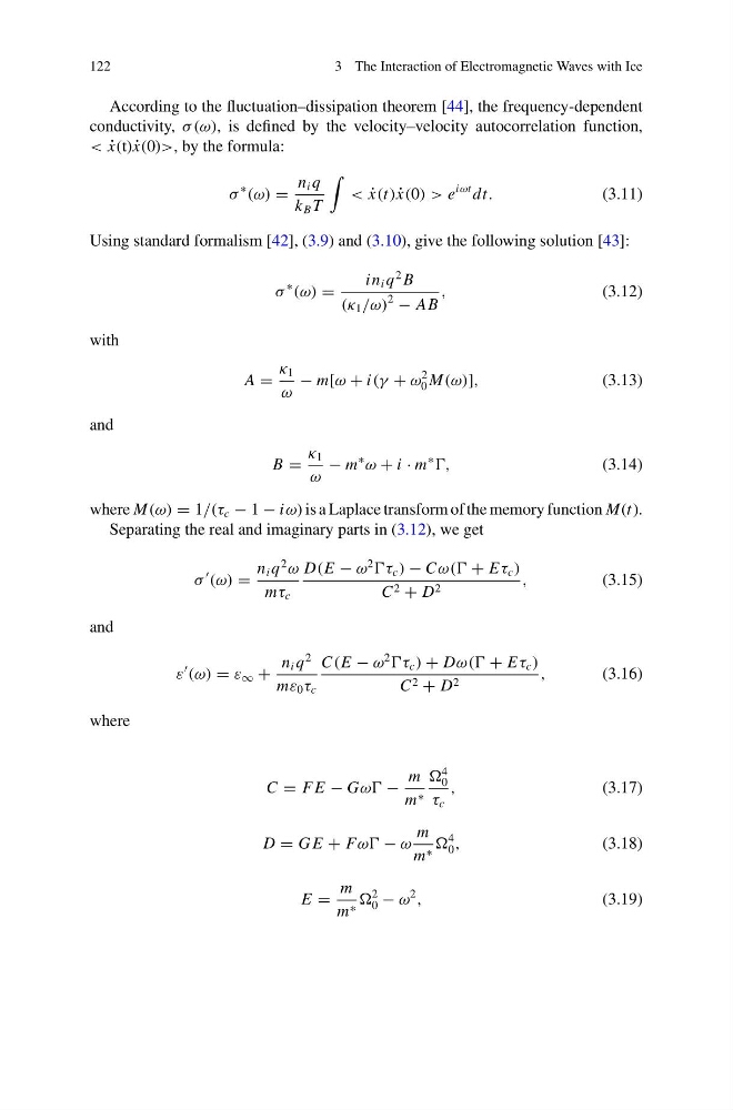
According to the fluctuation–dissipation theorem [44], the frequency-dependent
conductivity, σ (ω), is defined by the velocity–velocity autocorrelation function,
< ˙
x(t) ˙
x(0)>, by the formula:
σ
∗
(ω) =
n i q
k B T
< ˙
x(t) ˙
x(0) > e
iωt dt.
(3.11)
Using standard formalism [42], (3.9) and (3.10), give the following solution [43]:
σ
∗
(ω) =
in i q
2 B
(κ 1 /ω)
2
− AB
,
(3.12)
with
A =
κ 1
ω
− m[ω + i(γ + ω
2
0 M(ω)],
(3.13)
and
B =
κ 1
ω
− m
∗
ω + i · m
∗
,
(3.14)
where M(ω) = 1/(τ c − 1 − iω) is a Laplace transform of the memory function M(t).
Separating the real and imaginary parts in (3.12), we get
σ
(ω) =
n i q
2
ω
mτ c
D(E − ω
2
τ c ) − Cω(( + Eτ c )
C 2 + D 2
,
(3.15)
and
ε
(ω) = ε ∞ +
n i q
2
mε 0 τ c
C(E − ω
2
τ c ) + Dω(( + Eτ c )
C 2 + D 2
,
(3.16)
where
C = F E − Gωω −
m
m ∗
4
0
τ c
,
(3.17)
D = G E + Fωω − ω
m
m ∗
4
0 ,
(3.18)
E =
m
m ∗
2
0 − ω
2
,
(3.19)
3 The Interaction of Electromagnetic Waves with Ice
According to the fluctuation–dissipation theorem [44], the frequency-dependent
conductivity, σ (ω), is defined by the velocity–velocity autocorrelation function,
< ˙
x(t) ˙
x(0)>, by the formula:
σ
∗
(ω) =
n i q
k B T
< ˙
x(t) ˙
x(0) > e
iωt dt.
(3.11)
Using standard formalism [42], (3.9) and (3.10), give the following solution [43]:
σ
∗
(ω) =
in i q
2 B
(κ 1 /ω)
2
− AB
,
(3.12)
with
A =
κ 1
ω
− m[ω + i(γ + ω
2
0 M(ω)],
(3.13)
and
B =
κ 1
ω
− m
∗
ω + i · m
∗
,
(3.14)
where M(ω) = 1/(τ c − 1 − iω) is a Laplace transform of the memory function M(t).
Separating the real and imaginary parts in (3.12), we get
σ
(ω) =
n i q
2
ω
mτ c
D(E − ω
2
τ c ) − Cω(( + Eτ c )
C 2 + D 2
,
(3.15)
and
ε
(ω) = ε ∞ +
n i q
2
mε 0 τ c
C(E − ω
2
τ c ) + Dω(( + Eτ c )
C 2 + D 2
,
(3.16)
where
C = F E − Gωω −
m
m ∗
4
0
τ c
,
(3.17)
D = G E + Fωω − ω
m
m ∗
4
0 ,
(3.18)
E =
m
m ∗
2
0 − ω
2
,
(3.19)