

66
Biomedical Signal and Image Processing
f(x, y)
h(x, y)
Δ
g(x, y)
2
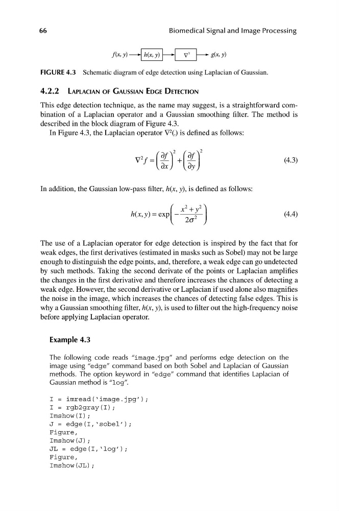
FIGURE 4.3 Schematic diagram of edge detection using Laplacian of Gaussian.
4.2.2 LAPLACIAN OF GAUSSIAN EDGE DETECTION
This edge detection technique, as the name may suggest, is a straightforward combination of a Laplacian operator and a Gaussian smoothing filter. The method is
described in the block diagram of Figure 4.3.
In Figure 4.3, the Laplacian operator ∇ 2 (.) is defined as follows:
2
⎛ ∂f ⎞
2
⎛ ∂f ⎞
2
∇ f =
+
(4.3)
⎝ ⎜ ∂x ⎠ ⎟ ⎝ ⎜ ∂y ⎠ ⎟
In addition, the Gaussian low-pass filter, h(x, y), is defined as follows:
⎛ x
2
+ y
2
⎞
h( , )
x y = exp −
2
(4.4)
⎝ ⎜
2s ⎠ ⎟
The use of a Laplacian operator for edge detection is inspired by the fact that for
weak edges, the first derivatives (estimated in masks such as Sobel) may not be large
enough to distinguish the edge points, and, therefore, a weak edge can go undetected
by such methods. Taking the second derivate of the points or Laplacian amplifies
the changes in the first derivative and therefore increases the chances of detecting a
weak edge. However, the second derivative or Laplacian if used alone also magnifies
the noise in the image, which increases the chances of detecting false edges. This is
why a Gaussian smoothing filter, h(x, y), is used to filter out the high-frequency noise
before applying Laplacian operator.
Example 4.3
The following code reads “image.jpg” and performs edge detection on the
image using “edge” command based on both Sobel and Laplacian of Gaussian
methods. The option keyword in “edge” command that identifies Laplacian of
Gaussian method is “log”.
I = imread(‘image.jpg’);
I = rgb2gray(I);
Imshow(I);
J = edge(I,‘sobel’);
Figure,
Imshow(J);
JL = edge(I,‘log’);
Figure,
Imshow(JL);
Biomedical Signal and Image Processing
f(x, y)
h(x, y)
Δ
g(x, y)
2
FIGURE 4.3 Schematic diagram of edge detection using Laplacian of Gaussian.
4.2.2 LAPLACIAN OF GAUSSIAN EDGE DETECTION
This edge detection technique, as the name may suggest, is a straightforward combination of a Laplacian operator and a Gaussian smoothing filter. The method is
described in the block diagram of Figure 4.3.
In Figure 4.3, the Laplacian operator ∇ 2 (.) is defined as follows:
2
⎛ ∂f ⎞
2
⎛ ∂f ⎞
2
∇ f =
+
(4.3)
⎝ ⎜ ∂x ⎠ ⎟ ⎝ ⎜ ∂y ⎠ ⎟
In addition, the Gaussian low-pass filter, h(x, y), is defined as follows:
⎛ x
2
+ y
2
⎞
h( , )
x y = exp −
2
(4.4)
⎝ ⎜
2s ⎠ ⎟
The use of a Laplacian operator for edge detection is inspired by the fact that for
weak edges, the first derivatives (estimated in masks such as Sobel) may not be large
enough to distinguish the edge points, and, therefore, a weak edge can go undetected
by such methods. Taking the second derivate of the points or Laplacian amplifies
the changes in the first derivative and therefore increases the chances of detecting a
weak edge. However, the second derivative or Laplacian if used alone also magnifies
the noise in the image, which increases the chances of detecting false edges. This is
why a Gaussian smoothing filter, h(x, y), is used to filter out the high-frequency noise
before applying Laplacian operator.
Example 4.3
The following code reads “image.jpg” and performs edge detection on the
image using “edge” command based on both Sobel and Laplacian of Gaussian
methods. The option keyword in “edge” command that identifies Laplacian of
Gaussian method is “log”.
I = imread(‘image.jpg’);
I = rgb2gray(I);
Imshow(I);
J = edge(I,‘sobel’);
Figure,
Imshow(J);
JL = edge(I,‘log’);
Figure,
Imshow(JL);