22
Biomedical Signal and Image Processing
3
2
1
0
–1
–2
–3
x(t)
0
1
2
3
4
5
6
7
8
9
1 0
Time t
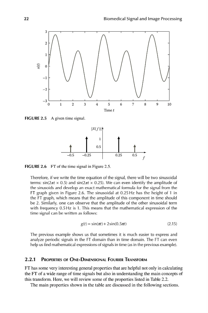
FIGURE 2.5 A given time signal.
1
0.5
|X( f )|
f
–0.5
–0.25
0.5
0.25
FIGURE 2.6 FT of the time signal in Figure 2.5.
Therefore, if we write the time equation of the signal, there will be two sinusoidal
terms: sin(2πt × 0.5) and sin(2πt × 0.25). We can even identify the amplitude of
the sinusoids and develop an exact mathematical formula for the signal from the
FT graph given in Figure 2.6. The sinusoidal at 0.25 Hz has the height of 1 in
the FT graph, which means that the amplitude of this component in time should
be 2. Similarly, one can observe that the amplitude of the other sinusoidal term
with frequency 0.5 Hz is 1. This means that the mathematical expression of the
time signal can be written as follows:
g t
( ) = sin( t) + 2sin( . pt)
(2.15)
p
0 5
The previous example shows us that sometimes it is much easier to express and
analyze periodic signals in the FT domain than in time domain. The FT can even
help us find mathematical expressions of signals in time (as in the previous example).
2.2.1 PROPERTIES OF ONE-DIMENSIONAL FOURIER TRANSFORM
FT has some very interesting general properties that are helpful not only in calculating
the FT of a wide range of time signals but also in understanding the main concepts of
this transform. Here, we will review some of the properties listed in Table 2.2.
The main properties shown in the table are discussed in the following sections.