

23
Fourier Transform
TABLE 2.2
Properties of 1-D FT
Time Function
dg t
( )
dt
g(t − t 0 )
j f t
2p 0
e
g t
( )
g 1 (t) × g 2 (t)
g 1 (t) × g 2 (t)
tg(t)
+∞
2
g t
( ) dt
∫
−∞
ag 1 (t) + bg 2 (t)
FT
( j2πf )G( f )
p 0
e
( )
2 ft G f
G( f − f 0 )
G 1 ( f ) × G 2 ( f )
G 1 ( f ) × G 2 ( f )
j dG f
( )
2p df
+∞
2
G f
( ) df
∫
−∞
aG 1 ( f ) + bG 2 ( f )
2.2.1.1 Signal Shift
According to this property, if a signal is shifted in time, the magnitude of the FT remains
the same (for all frequencies). Specifically, for a signal g(t) and an arbitrary time shift t 0 ,
j ft G f
FT g t
{ ( − t 0 )} = e
2p 0 ( )
(2.16)
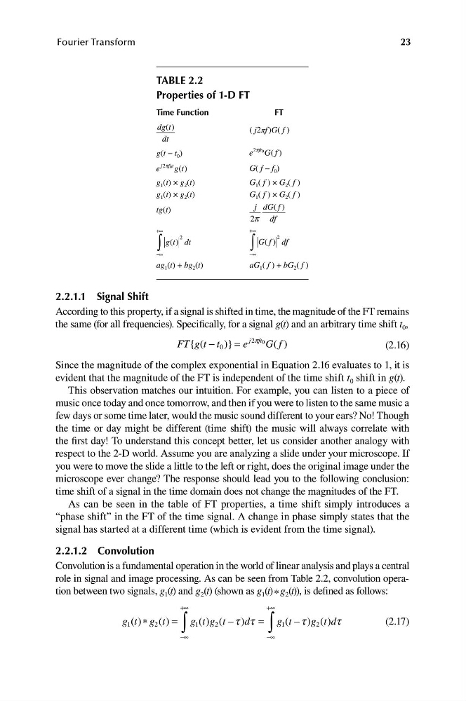
Since the magnitude of the complex exponential in Equation 2.16 evaluates to 1, it is
evident that the magnitude of the FT is independent of the time shift t 0 shift in g(t).
This observation matches our intuition. For example, you can listen to a piece of
music once today and once tomorrow, and then if you were to listen to the same music a
few days or some time later, would the music sound different to your ears? No! Though
the time or day might be different (time shift) the music will always correlate with
the first day! To understand this concept better, let us consider another analogy with
respect to the 2-D world. Assume you are analyzing a slide under your microscope. If
you were to move the slide a little to the left or right, does the original image under the
microscope ever change? The response should lead you to the following conclusion:
time shift of a signal in the time domain does not change the magnitudes of the FT.
As can be seen in the table of FT properties, a time shift simply introduces a
“phase shift” in the FT of the time signal. A change in phase simply states that the
signal has started at a different time (which is evident from the time signal).
2.2.1.2 Convolution
Convolution is a fundamental operation in the world of linear analysis and plays a central
role in signal and image processing. As can be seen from Table 2.2, convolution operation between two signals, g 1 (t) and g 2 (t) (shown as g 1 (t) * g 2 (t)), is defined as follows:
+∞
+∞
g t ∗ g ( ) = g t g (t − )d = g (t − t )g t d t
1 ( ) 2 t
1 ( ) 2
t t
1
2 ( )
(2.17)
∫
∫
−∞
−∞
Fourier Transform
TABLE 2.2
Properties of 1-D FT
Time Function
dg t
( )
dt
g(t − t 0 )
j f t
2p 0
e
g t
( )
g 1 (t) × g 2 (t)
g 1 (t) × g 2 (t)
tg(t)
+∞
2
g t
( ) dt
∫
−∞
ag 1 (t) + bg 2 (t)
FT
( j2πf )G( f )
p 0
e
( )
2 ft G f
G( f − f 0 )
G 1 ( f ) × G 2 ( f )
G 1 ( f ) × G 2 ( f )
j dG f
( )
2p df
+∞
2
G f
( ) df
∫
−∞
aG 1 ( f ) + bG 2 ( f )
2.2.1.1 Signal Shift
According to this property, if a signal is shifted in time, the magnitude of the FT remains
the same (for all frequencies). Specifically, for a signal g(t) and an arbitrary time shift t 0 ,
j ft G f
FT g t
{ ( − t 0 )} = e
2p 0 ( )
(2.16)
Since the magnitude of the complex exponential in Equation 2.16 evaluates to 1, it is
evident that the magnitude of the FT is independent of the time shift t 0 shift in g(t).
This observation matches our intuition. For example, you can listen to a piece of
music once today and once tomorrow, and then if you were to listen to the same music a
few days or some time later, would the music sound different to your ears? No! Though
the time or day might be different (time shift) the music will always correlate with
the first day! To understand this concept better, let us consider another analogy with
respect to the 2-D world. Assume you are analyzing a slide under your microscope. If
you were to move the slide a little to the left or right, does the original image under the
microscope ever change? The response should lead you to the following conclusion:
time shift of a signal in the time domain does not change the magnitudes of the FT.
As can be seen in the table of FT properties, a time shift simply introduces a
“phase shift” in the FT of the time signal. A change in phase simply states that the
signal has started at a different time (which is evident from the time signal).
2.2.1.2 Convolution
Convolution is a fundamental operation in the world of linear analysis and plays a central
role in signal and image processing. As can be seen from Table 2.2, convolution operation between two signals, g 1 (t) and g 2 (t) (shown as g 1 (t) * g 2 (t)), is defined as follows:
+∞
+∞
g t ∗ g ( ) = g t g (t − )d = g (t − t )g t d t
1 ( ) 2 t
1 ( ) 2
t t
1
2 ( )
(2.17)
∫
∫
−∞
−∞