

21
Fourier Transform
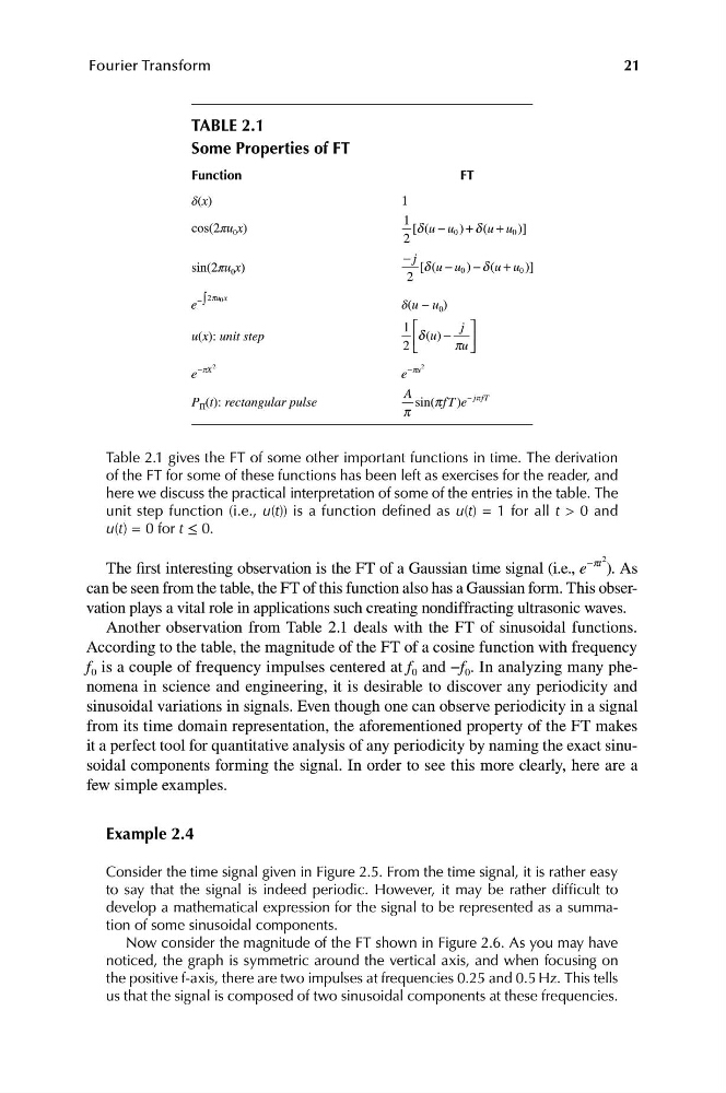
TABLE 2.1
Some Properties of FT
Function
δ(x)
cos(2πu 0 x)
sin(2πu 0 x)
u x
−∫ 2p 0
e
u(x): unit step
−pX 2
e
P Π (t): rectangular pulse
FT
1
1 [ (u u
d − 0 ) + d ( + 0 )]
u u
2
− j [ (u u 0
d −
+ 0 )]
) − d (u u
2
δ(u − u 0 )
1 ⎡
j ⎤
d ( ) −
u
⎢
⎥
2 ⎣
pu ⎦
−pu 2
e
A
)
− p
j fT
sin(pfT e
p
Table 2.1 gives the FT of some other important functions in time. The derivation
of the FT for some of these functions has been left as exercises for the reader, and
here we discuss the practical interpretation of some of the entries in the table. The
unit step function (i.e., u(t)) is a function defined as u(t) = 1 for all t > 0 and
u(t) = 0 for t ≤ 0.
−pt
2
The first interesting observation is the FT of a Gaussian time signal (i.e., e ). As
can be seen from the table, the FT of this function also has a Gaussian form. This observation plays a vital role in applications such creating nondiffracting ultrasonic waves.
Another observation from Table 2.1 deals with the FT of sinusoidal functions.
According to the table, the magnitude of the FT of a cosine function with frequency
f 0 is a couple of frequency impulses centered at f 0 and −f 0 . In analyzing many phenomena in science and engineering, it is desirable to discover any periodicity and
sinusoidal variations in signals. Even though one can observe periodicity in a signal
from its time domain representation, the aforementioned property of the FT makes
it a perfect tool for quantitative analysis of any periodicity by naming the exact sinusoidal components forming the signal. In order to see this more clearly, here are a
few simple examples.
Example 2.4
Consider the time signal given in Figure 2.5. From the time signal, it is rather easy
to say that the signal is indeed periodic. However, it may be rather difficult to
develop a mathematical expression for the signal to be represented as a summation of some sinusoidal components.
Now consider the magnitude of the FT shown in Figure 2.6. As you may have
noticed, the graph is symmetric around the vertical axis, and when focusing on
the positive f-axis, there are two impulses at frequencies 0.25 and 0.5 Hz. This tells
us that the signal is composed of two sinusoidal components at these frequencies.
Fourier Transform
TABLE 2.1
Some Properties of FT
Function
δ(x)
cos(2πu 0 x)
sin(2πu 0 x)
u x
−∫ 2p 0
e
u(x): unit step
−pX 2
e
P Π (t): rectangular pulse
FT
1
1 [ (u u
d − 0 ) + d ( + 0 )]
u u
2
− j [ (u u 0
d −
+ 0 )]
) − d (u u
2
δ(u − u 0 )
1 ⎡
j ⎤
d ( ) −
u
⎢
⎥
2 ⎣
pu ⎦
−pu 2
e
A
)
− p
j fT
sin(pfT e
p
Table 2.1 gives the FT of some other important functions in time. The derivation
of the FT for some of these functions has been left as exercises for the reader, and
here we discuss the practical interpretation of some of the entries in the table. The
unit step function (i.e., u(t)) is a function defined as u(t) = 1 for all t > 0 and
u(t) = 0 for t ≤ 0.
−pt
2
The first interesting observation is the FT of a Gaussian time signal (i.e., e ). As
can be seen from the table, the FT of this function also has a Gaussian form. This observation plays a vital role in applications such creating nondiffracting ultrasonic waves.
Another observation from Table 2.1 deals with the FT of sinusoidal functions.
According to the table, the magnitude of the FT of a cosine function with frequency
f 0 is a couple of frequency impulses centered at f 0 and −f 0 . In analyzing many phenomena in science and engineering, it is desirable to discover any periodicity and
sinusoidal variations in signals. Even though one can observe periodicity in a signal
from its time domain representation, the aforementioned property of the FT makes
it a perfect tool for quantitative analysis of any periodicity by naming the exact sinusoidal components forming the signal. In order to see this more clearly, here are a
few simple examples.
Example 2.4
Consider the time signal given in Figure 2.5. From the time signal, it is rather easy
to say that the signal is indeed periodic. However, it may be rather difficult to
develop a mathematical expression for the signal to be represented as a summation of some sinusoidal components.
Now consider the magnitude of the FT shown in Figure 2.6. As you may have
noticed, the graph is symmetric around the vertical axis, and when focusing on
the positive f-axis, there are two impulses at frequencies 0.25 and 0.5 Hz. This tells
us that the signal is composed of two sinusoidal components at these frequencies.