

326
Biomedical Signal and Image Processing
Similarly, we can calculate the reflected wave front at the separation surface as
follows:
y 1 ( )
t = p 1 ( )
t n x y
( , )
(16.37)
Assuming the delay in p 1 (t) relative to p(t), ψ 1 (t) can be rewritten as follows:
⎛
x ⎞
y 1 ( )
t = p ⎜ t − ⎟ n x
( , y )
(16.38)
⎝ V ⎠
Now, knowing that ψ(t) is indeed the delayed version of ψ 1 (t), we can express the
mathematical formulation of the returned pulse as follows:
⎛
x ⎞
y ( )
t = p ⎜ t − 2 ⎟ n x
( , y )
(16.39)
⎝
V ⎠
In the preceding formulation, we assumed no attenuation throughout the process.
Now, in order to have a more accurate formulation of the system, we modify the preceding equations to incorporate attenuation. In formulation reflection tomography,
the attenuation effect is often modeled using an experimental rule. This rule states
that ultrasound waves traveling a given distance x are attenuated proportional to
1 . This reciprocal of square root law simplifies the formulation and is known to
x
be accurate assumption in almost all biological tissues. Using this rule and assuming
that the wave is traveling in x direction, Equations 16.38 and 16.39 can be rewritten
as follows:
⎛
x ⎞ n x
( , y )
y 1 ( )
t = p ⎜ t − ⎟ .
(16.40)
⎝ V ⎠
x
⎛
x ⎞ n x
( , y )
y ( )
t = p ⎜ t − 2 ⎟ .
(16.41)
⎝
V ⎠
x
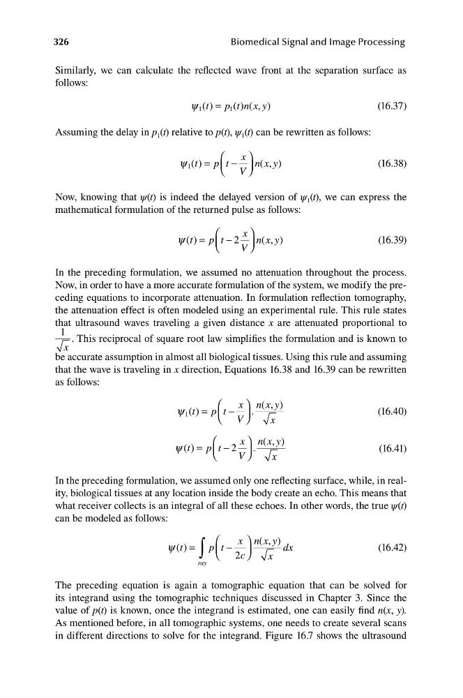
In the preceding formulation, we assumed only one reflecting surface, while, in reality, biological tissues at any location inside the body create an echo. This means that
what receiver collects is an integral of all these echoes. In other words, the true ψ(t)
can be modeled as follows:
⎛
x ⎞ n x
( , y )
y ( )
t =
∫
p ⎜ t − ⎟
dx
(16.42)
⎝ 2c ⎠
x
ray
The preceding equation is again a tomographic equation that can be solved for
its integrand using the tomographic techniques discussed in Chapter 3. Since the
value of p(t) is known, once the integrand is estimated, one can easily find n(x, y).
As mentioned before, in all tomographic systems, one needs to create several scans
in different directions to solve for the integrand. Figure 16.7 shows the ultrasound
Biomedical Signal and Image Processing
Similarly, we can calculate the reflected wave front at the separation surface as
follows:
y 1 ( )
t = p 1 ( )
t n x y
( , )
(16.37)
Assuming the delay in p 1 (t) relative to p(t), ψ 1 (t) can be rewritten as follows:
⎛
x ⎞
y 1 ( )
t = p ⎜ t − ⎟ n x
( , y )
(16.38)
⎝ V ⎠
Now, knowing that ψ(t) is indeed the delayed version of ψ 1 (t), we can express the
mathematical formulation of the returned pulse as follows:
⎛
x ⎞
y ( )
t = p ⎜ t − 2 ⎟ n x
( , y )
(16.39)
⎝
V ⎠
In the preceding formulation, we assumed no attenuation throughout the process.
Now, in order to have a more accurate formulation of the system, we modify the preceding equations to incorporate attenuation. In formulation reflection tomography,
the attenuation effect is often modeled using an experimental rule. This rule states
that ultrasound waves traveling a given distance x are attenuated proportional to
1 . This reciprocal of square root law simplifies the formulation and is known to
x
be accurate assumption in almost all biological tissues. Using this rule and assuming
that the wave is traveling in x direction, Equations 16.38 and 16.39 can be rewritten
as follows:
⎛
x ⎞ n x
( , y )
y 1 ( )
t = p ⎜ t − ⎟ .
(16.40)
⎝ V ⎠
x
⎛
x ⎞ n x
( , y )
y ( )
t = p ⎜ t − 2 ⎟ .
(16.41)
⎝
V ⎠
x
In the preceding formulation, we assumed only one reflecting surface, while, in reality, biological tissues at any location inside the body create an echo. This means that
what receiver collects is an integral of all these echoes. In other words, the true ψ(t)
can be modeled as follows:
⎛
x ⎞ n x
( , y )
y ( )
t =
∫
p ⎜ t − ⎟
dx
(16.42)
⎝ 2c ⎠
x
ray
The preceding equation is again a tomographic equation that can be solved for
its integrand using the tomographic techniques discussed in Chapter 3. Since the
value of p(t) is known, once the integrand is estimated, one can easily find n(x, y).
As mentioned before, in all tomographic systems, one needs to create several scans
in different directions to solve for the integrand. Figure 16.7 shows the ultrasound