

322
Biomedical Signal and Image Processing
In the interface of the water layer and the tissue, only a portion of the signal energy
gets to enter the tissue. This portion of the signal, Z 2 (f), can be calculated using the
transmittance factor between water and tissue, A WT , as follows:
Z f
( ) = A Z f
2
WT 1 ( )
(16.18)
Now the pulse that has entered the tissue gets attenuated and delayed throughout the tissue. Since we are not assuming that the tissue is a homogeneous environment, the values
of attenuation and delay must be calculated for each point and then integrated over the
entire linear path to provide the total attenuation and delay across the tissue. This means
that the signal at the far right side of the tissue, Z 3 (f), can be calculated as follows:
l
l
− j b x y f dx
, )
− a ( , , ) x
( ,
x y f d
∫
∫
Z f
( ) = e
0
e
0
Z f
3
2 ( )
(16.19)
As can be seen in Equation 16.19, α(x, y, f) and β(x, y, f) are assumed to depend on
the exact location of the point as well as the exact frequency. The next step is the
transmittance of the signal from the far right side of the tissue to the water on the
receiver side of the system, which can be represented by the following:
Z f
( ) = A Z f
W
( )
4
T
3
(16.20)
where A TW is the transmittance factor from the tissue to water. As in the transmitter
side, the signal is both attenuated and delayed while passing through the water interface with thickness l W2 , i.e., the pressure signal on the far right hand side of the water
interface, Y a (f), will be as follows:
− jb W ( )
f l W 2 −a W ( ) W 2
Y f
( ) = e
e
f l Z f
a
4 ( )
(16.21)
Finally, the conversion of the mechanical pressure Y a (f) to electric signal Y(f), as
shown in Figure 16.5, can be formulated as another linear system with an impulse
function H 2 (f) as follows:
Y f = H f Y f
( )
(16.22)
( )
2 ( ) a
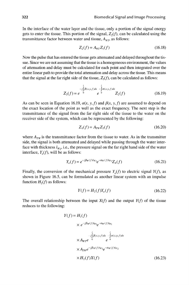
The overall relationship between the input X(f) and the output Y(f) of the tissue
reduces to the following:
Y f = H f
( )
1 ( )
− jb W ( )
f l W1 −a W ( )
f l W1
× e
e
l
l
− j b ( ,
x y f dx
)
− a ( ,y, ) x
,
x y f d
∫
∫
× A e
0
e
0
W T
− jb W ( )
f l W −a W f l W
( )
× A e
2
e
2
TW
× H f X f
( )
2 ( )
(16.23)
Biomedical Signal and Image Processing
In the interface of the water layer and the tissue, only a portion of the signal energy
gets to enter the tissue. This portion of the signal, Z 2 (f), can be calculated using the
transmittance factor between water and tissue, A WT , as follows:
Z f
( ) = A Z f
2
WT 1 ( )
(16.18)
Now the pulse that has entered the tissue gets attenuated and delayed throughout the tissue. Since we are not assuming that the tissue is a homogeneous environment, the values
of attenuation and delay must be calculated for each point and then integrated over the
entire linear path to provide the total attenuation and delay across the tissue. This means
that the signal at the far right side of the tissue, Z 3 (f), can be calculated as follows:
l
l
− j b x y f dx
, )
− a ( , , ) x
( ,
x y f d
∫
∫
Z f
( ) = e
0
e
0
Z f
3
2 ( )
(16.19)
As can be seen in Equation 16.19, α(x, y, f) and β(x, y, f) are assumed to depend on
the exact location of the point as well as the exact frequency. The next step is the
transmittance of the signal from the far right side of the tissue to the water on the
receiver side of the system, which can be represented by the following:
Z f
( ) = A Z f
W
( )
4
T
3
(16.20)
where A TW is the transmittance factor from the tissue to water. As in the transmitter
side, the signal is both attenuated and delayed while passing through the water interface with thickness l W2 , i.e., the pressure signal on the far right hand side of the water
interface, Y a (f), will be as follows:
− jb W ( )
f l W 2 −a W ( ) W 2
Y f
( ) = e
e
f l Z f
a
4 ( )
(16.21)
Finally, the conversion of the mechanical pressure Y a (f) to electric signal Y(f), as
shown in Figure 16.5, can be formulated as another linear system with an impulse
function H 2 (f) as follows:
Y f = H f Y f
( )
(16.22)
( )
2 ( ) a
The overall relationship between the input X(f) and the output Y(f) of the tissue
reduces to the following:
Y f = H f
( )
1 ( )
− jb W ( )
f l W1 −a W ( )
f l W1
× e
e
l
l
− j b ( ,
x y f dx
)
− a ( ,y, ) x
,
x y f d
∫
∫
× A e
0
e
0
W T
− jb W ( )
f l W −a W f l W
( )
× A e
2
e
2
TW
× H f X f
( )
2 ( )
(16.23)