

323
Ultrasound Imaging
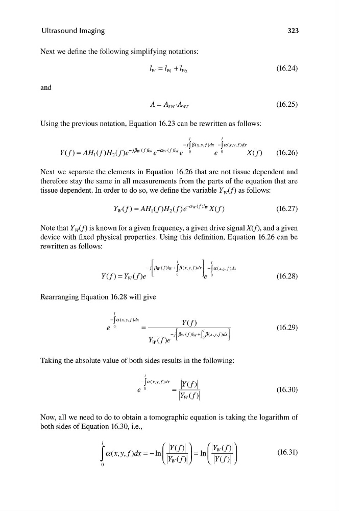
Next we define the following simplifying notations:
l W = l W 1 + l W 2
(16.24)
and
A A
= TW . A WT
(16.25)
Using the previous notation, Equation 16.23 can be rewritten as follows:
l
l
− j ∫ b ( ,
xy, f) dx − ∫ a ( ,
xy f d
) x
Y f
( ) = AH ( )
f H ( )
f e
− jb W ( )
f l W e
−a W ( )
f l W
1
2
e
0
e
0
X f
( )
(16.26)
Next we separate the elements in Equation 16.26 that are not tissue dependent and
therefore stay the same in all measurements from the parts of the equation that are
tissue dependent. In order to do so, we define the variable Y W (f) as follows:
Y f
W ( ) = AH ( )
f H ( )
f e
−a W ( )
f l W ( )
1
2
X f
(16.27)
Note that Y W (f) is known for a given frequency, a given drive signal X(f), and a given
device with fixed physical properties. Using this definition, Equation 16.26 can be
rewritten as follows:
⎡
l
⎤
l
− j ⎢ b W ( )
f l W + ∫ b ( x ,y , f) d x ⎥ − ∫ a ( ,
x y, f )dx
⎢
⎥
Y f
( ) = Y ( )
f e
⎣
0
⎦
0
W
e
(16.28)
Rearranging Equation 16.28 will give
l
− ∫ a ( ,
x y, f ) dx
0
Y f
( )
e
=
16.29)
⎡
l
(
⎤
− j b
⎢ W ( )
f l W + ∫ b ( x ,y , f) d x
( )
0
⎥
Y f
⎦
W
e
⎣
Taking the absolute value of both sides results in the following:
l
− ∫ a ( ,
x y, f ) dx
Y f
( )
e
0
=
(16.30)
Y f
W ( )
Now, all we need to do to obtain a tomographic equation is taking the logarithm of
both sides of Equation 16.30, i.e.,
∫
l
⎛ Y f
( ) ⎞
⎛ Y f
( ) ⎞
a( ,
x y, f ) dx = − ln
=
W
(16.31)
⎜
⎟ ln ⎜
⎟
⎝ Y f
W ( ) ⎠
⎝ Y f
( ) ⎠
0
, ,
Ultrasound Imaging
Next we define the following simplifying notations:
l W = l W 1 + l W 2
(16.24)
and
A A
= TW . A WT
(16.25)
Using the previous notation, Equation 16.23 can be rewritten as follows:
l
l
− j ∫ b ( ,
xy, f) dx − ∫ a ( ,
xy f d
) x
Y f
( ) = AH ( )
f H ( )
f e
− jb W ( )
f l W e
−a W ( )
f l W
1
2
e
0
e
0
X f
( )
(16.26)
Next we separate the elements in Equation 16.26 that are not tissue dependent and
therefore stay the same in all measurements from the parts of the equation that are
tissue dependent. In order to do so, we define the variable Y W (f) as follows:
Y f
W ( ) = AH ( )
f H ( )
f e
−a W ( )
f l W ( )
1
2
X f
(16.27)
Note that Y W (f) is known for a given frequency, a given drive signal X(f), and a given
device with fixed physical properties. Using this definition, Equation 16.26 can be
rewritten as follows:
⎡
l
⎤
l
− j ⎢ b W ( )
f l W + ∫ b ( x ,y , f) d x ⎥ − ∫ a ( ,
x y, f )dx
⎢
⎥
Y f
( ) = Y ( )
f e
⎣
0
⎦
0
W
e
(16.28)
Rearranging Equation 16.28 will give
l
− ∫ a ( ,
x y, f ) dx
0
Y f
( )
e
=
16.29)
⎡
l
(
⎤
− j b
⎢ W ( )
f l W + ∫ b ( x ,y , f) d x
( )
0
⎥
Y f
⎦
W
e
⎣
Taking the absolute value of both sides results in the following:
l
− ∫ a ( ,
x y, f ) dx
Y f
( )
e
0
=
(16.30)
Y f
W ( )
Now, all we need to do to obtain a tomographic equation is taking the logarithm of
both sides of Equation 16.30, i.e.,
∫
l
⎛ Y f
( ) ⎞
⎛ Y f
( ) ⎞
a( ,
x y, f ) dx = − ln
=
W
(16.31)
⎜
⎟ ln ⎜
⎟
⎝ Y f
W ( ) ⎠
⎝ Y f
( ) ⎠
0
, ,