

258
Biomedical Signal and Image Processing
As can be seen in Figure 13.9, one-dimensional (1-D) FT of the projection function
for beams θ = 0 (with x-axis in space domain) gives the 2-D FT of f(x, y) on v = 0 axis.
In other words, one can simply conduct one set of parallel scans along the x-axis and
calculate the values of the FT of the resulting projection function to obtain the values
of F(u, v) along the u-axis. This is a big step toward our goal of estimating F(u, v), but
having F(u, v) only along one axis is not sufficient to form f(x, y), i.e., we need F(u, v)
all over the 2-D frequency domain to create a better estimation of F(u, v). Repeating
measurement at different angles will produce the values of F(u, v) on different lines in
the (u, v) plane. This phenomenon is often referred to as Fourier slice theorem.
13.3 FOURIER SLICE THEOREM
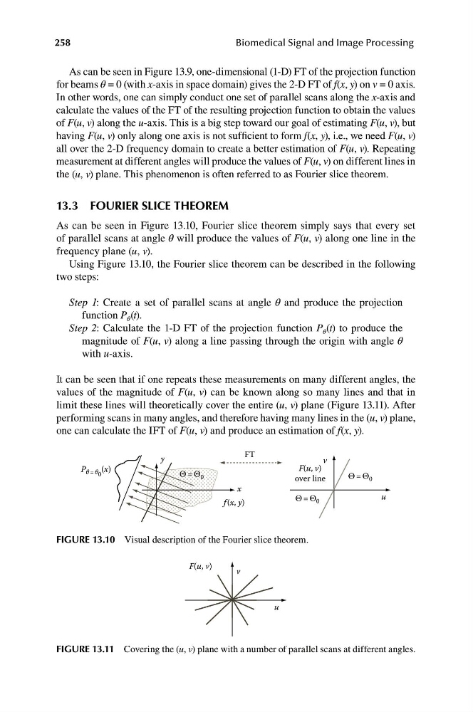
As can be seen in Figure 13.10, Fourier slice theorem simply says that every set
of parallel scans at angle θ will produce the values of F(u, v) along one line in the
frequency plane (u, v).
Using Figure 13.10, the Fourier slice theorem can be described in the following
two steps:
Step 1: Create a set of parallel scans at angle θ and produce the projection
function P θ (t).
Step 2: Calculate the 1-D FT of the projection function P θ (t) to produce the
magnitude of F(u, v) along a line passing through the origin with angle θ
with u-axis.
It can be seen that if one repeats these measurements on many different angles, the
values of the magnitude of F(u, v) can be known along so many lines and that in
limit these lines will theoretically cover the entire (u, v) plane (Figure 13.11). After
performing scans in many angles, and therefore having many lines in the (u, v) plane,
one can calculate the IFT of F(u, v) and produce an estimation of f(x, y).
Θ = Θ 0
f (x, y)
x
y
FT
v
F(u, v)
P θ = θ 0 (x)
Θ = Θ 0
over line
Θ = Θ 0
u
FIGURE 13.10 Visual description of the Fourier slice theorem.
F(u, v)
v
u
FIGURE 13.11 Covering the (u, v) plane with a number of parallel scans at different angles.
Biomedical Signal and Image Processing
As can be seen in Figure 13.9, one-dimensional (1-D) FT of the projection function
for beams θ = 0 (with x-axis in space domain) gives the 2-D FT of f(x, y) on v = 0 axis.
In other words, one can simply conduct one set of parallel scans along the x-axis and
calculate the values of the FT of the resulting projection function to obtain the values
of F(u, v) along the u-axis. This is a big step toward our goal of estimating F(u, v), but
having F(u, v) only along one axis is not sufficient to form f(x, y), i.e., we need F(u, v)
all over the 2-D frequency domain to create a better estimation of F(u, v). Repeating
measurement at different angles will produce the values of F(u, v) on different lines in
the (u, v) plane. This phenomenon is often referred to as Fourier slice theorem.
13.3 FOURIER SLICE THEOREM
As can be seen in Figure 13.10, Fourier slice theorem simply says that every set
of parallel scans at angle θ will produce the values of F(u, v) along one line in the
frequency plane (u, v).
Using Figure 13.10, the Fourier slice theorem can be described in the following
two steps:
Step 1: Create a set of parallel scans at angle θ and produce the projection
function P θ (t).
Step 2: Calculate the 1-D FT of the projection function P θ (t) to produce the
magnitude of F(u, v) along a line passing through the origin with angle θ
with u-axis.
It can be seen that if one repeats these measurements on many different angles, the
values of the magnitude of F(u, v) can be known along so many lines and that in
limit these lines will theoretically cover the entire (u, v) plane (Figure 13.11). After
performing scans in many angles, and therefore having many lines in the (u, v) plane,
one can calculate the IFT of F(u, v) and produce an estimation of f(x, y).
Θ = Θ 0
f (x, y)
x
y
FT
v
F(u, v)
P θ = θ 0 (x)
Θ = Θ 0
over line
Θ = Θ 0
u
FIGURE 13.10 Visual description of the Fourier slice theorem.
F(u, v)
v
u
FIGURE 13.11 Covering the (u, v) plane with a number of parallel scans at different angles.