

257
Principles of Computed Tomography
In order to see how FT is used for this purpose, first consider FT of the projection
function along a particular line for a fixed θ, i.e.,
+∞
S w
( ) = P t e
( )
− j w
2p t t
(13.7)
q
q
d
∫
−∞
Also, consider the 2-D FT of the object function f(x, y):
+∞ +∞
− j2p (ux v
+ y)
F u v =
f x y e
, )
dxdy
(13.8)
( , )
(
∫ ∫
−∞ −∞
Now, for v = 0, FT along the horizontal frequency coordinate becomes
+∞ +∞
+ +∞ +∞
j ux
− 2p x
− 2p
j u
F u 0 =
f x y e
)
dxdy =
f x y d
, ) y e
dx
(13.9)
( , )
( ,
⎜
(
⎟
∫ ∫
∫
⎛
⎜ ∫
⎞
⎟
−∞ −∞
−∞ ⎝ −∞
⎠
+∞
But from Equation 13.5, remember that P 0 ( )
f x y d
, ) y
q = x
(
, which means
=
∫ −∞
Equation 13.9 can be rewritten as follows:
+∞
− j u
2p x
F u 0 = P =0 ( )
dx
(13.10)
( , )
∫
q
x e
−∞
+∞
j u
p x
Now, from Equation 13.7, we know that S q =0 u =
∫
P q =0 ( )
x e
− 2
dx
( )
, which means
−∞
F u 0 = S ( ) = FT P
( , ) q =0 u
{ q =0 ( )
x }
(13.11)
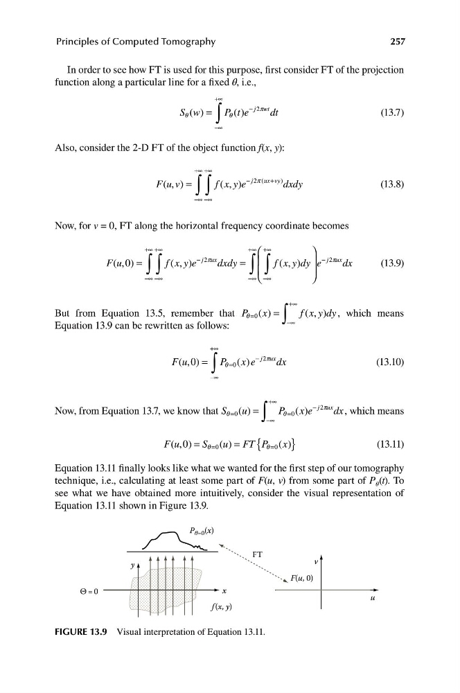
Equation 13.11 finally looks like what we wanted for the first step of our tomography
technique, i.e., calculating at least some part of F(u, v) from some part of P θ (t). To
see what we have obtained more intuitively, consider the visual representation of
Equation 13.11 shown in Figure 13.9.
f (x, y)
FT
F(u, 0)
v
u
x
P θ=0 (x)
Θ = 0
y
FIGURE 13.9 Visual interpretation of Equation 13.11.
Principles of Computed Tomography
In order to see how FT is used for this purpose, first consider FT of the projection
function along a particular line for a fixed θ, i.e.,
+∞
S w
( ) = P t e
( )
− j w
2p t t
(13.7)
q
q
d
∫
−∞
Also, consider the 2-D FT of the object function f(x, y):
+∞ +∞
− j2p (ux v
+ y)
F u v =
f x y e
, )
dxdy
(13.8)
( , )
(
∫ ∫
−∞ −∞
Now, for v = 0, FT along the horizontal frequency coordinate becomes
+∞ +∞
+ +∞ +∞
j ux
− 2p x
− 2p
j u
F u 0 =
f x y e
)
dxdy =
f x y d
, ) y e
dx
(13.9)
( , )
( ,
⎜
(
⎟
∫ ∫
∫
⎛
⎜ ∫
⎞
⎟
−∞ −∞
−∞ ⎝ −∞
⎠
+∞
But from Equation 13.5, remember that P 0 ( )
f x y d
, ) y
q = x
(
, which means
=
∫ −∞
Equation 13.9 can be rewritten as follows:
+∞
− j u
2p x
F u 0 = P =0 ( )
dx
(13.10)
( , )
∫
q
x e
−∞
+∞
j u
p x
Now, from Equation 13.7, we know that S q =0 u =
∫
P q =0 ( )
x e
− 2
dx
( )
, which means
−∞
F u 0 = S ( ) = FT P
( , ) q =0 u
{ q =0 ( )
x }
(13.11)
Equation 13.11 finally looks like what we wanted for the first step of our tomography
technique, i.e., calculating at least some part of F(u, v) from some part of P θ (t). To
see what we have obtained more intuitively, consider the visual representation of
Equation 13.11 shown in Figure 13.9.
f (x, y)
FT
F(u, 0)
v
u
x
P θ=0 (x)
Θ = 0
y
FIGURE 13.9 Visual interpretation of Equation 13.11.