

121
Other Signal and Image Processing Methods
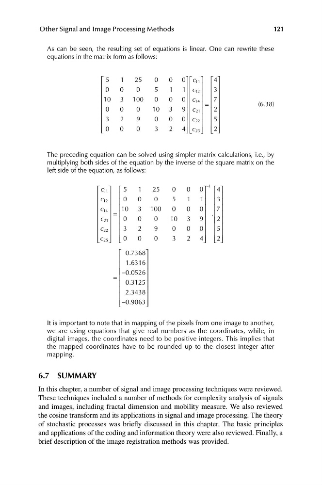
As can be seen, the resulting set of equations is linear. One can rewrite these
equations in the matrix form as follows:
⎡ 5
1
25
0
0 0 ⎤ ⎡c11 ⎤ ⎡4⎤
⎢
⎥ ⎢ ⎥ ⎢ ⎥
0
0
0
5
1 1 c
3
⎢
⎥ ⎢
12
⎥ ⎢ ⎥
⎢ 10 3 100
0
0 0 ⎥ ⎢ c ⎥ ⎢7 ⎥
⎢
⎥ ⎢
14 ⎥ = ⎢ ⎥
(6.38)
⎢ 0
0
0
10 3 9 ⎥ ⎢ c 21 ⎥ ⎢ 2 ⎥
⎢ 3
2
9
0
0 0 ⎥ ⎥ ⎢ c ⎥ ⎢
⎢
⎥ ⎢
22
5 ⎥
⎥ ⎢ ⎥
⎢ ⎣ 0
0
0
3
2 4 ⎦ ⎥ ⎣ ⎢c25 ⎦ ⎥ ⎢ ⎢ ⎣ 2 ⎥ ⎦
The preceding equation can be solved using simpler matrix calculations, i.e., by
multiplying both sides of the equation by the inverse of the square matrix on the
left side of the equation, as follows:
⎡ ⎤ ⎡
−
c 11
5
1
25
0
0 0 ⎤
1 ⎡4⎤
⎢ ⎥ ⎢
⎥ ⎢ ⎥
c 12
0
0
0
5
1 1
3
⎢ ⎥ ⎢
⎥ ⎢ ⎥
⎢ c 14 ⎥ ⎢ 10 3 100
0 0
0 0 ⎥ ⎢7 ⎥
⎢ ⎥ = ⎢
⎥ . ⎢ ⎥
⎢ c 21 ⎥ ⎢ 0
0
0
10 3 9 ⎥ ⎢ ⎢ 2 ⎥
⎢ c 22 ⎥ ⎢ 3
2
9
0
0 0 ⎥ ⎢ 5 ⎥
⎢ ⎥ ⎢
⎥ ⎢ ⎥
⎣ ⎢c25 ⎦ ⎥ ⎢ ⎣ 0
0
0
3
2 4 ⎥ ⎦ ⎣ ⎢2 ⎥ ⎦
⎡ 0 . 7368⎤
⎢
⎥
1 . 6316
⎢
⎥
⎢ ⎢ −0 . 0526⎥
= ⎢
⎥
⎢ 0 . 3125 ⎥
⎢ 2 . 3438 ⎥
⎢
⎥
⎢− .
⎦ ⎥
⎣ 0 9063
It is important to note that in mapping of the pixels from one image to another,
we are using equations that give real numbers as the coordinates, while, in
digital images, the coordinates need to be positive integers. This implies that
the mapped coordinates have to be rounded up to the closest integer after
mapping.
6.7 SUMMARY
In this chapter, a number of signal and image processing techniques were reviewed.
These techniques included a number of methods for complexity analysis of signals
and images, including fractal dimension and mobility measure. We also reviewed
the cosine transform and its applications in signal and image processing. The theory
of stochastic processes was briefly discussed in this chapter. The basic principles
and applications of the coding and information theory were also reviewed. Finally, a
brief description of the image registration methods was provided.
Other Signal and Image Processing Methods
As can be seen, the resulting set of equations is linear. One can rewrite these
equations in the matrix form as follows:
⎡ 5
1
25
0
0 0 ⎤ ⎡c11 ⎤ ⎡4⎤
⎢
⎥ ⎢ ⎥ ⎢ ⎥
0
0
0
5
1 1 c
3
⎢
⎥ ⎢
12
⎥ ⎢ ⎥
⎢ 10 3 100
0
0 0 ⎥ ⎢ c ⎥ ⎢7 ⎥
⎢
⎥ ⎢
14 ⎥ = ⎢ ⎥
(6.38)
⎢ 0
0
0
10 3 9 ⎥ ⎢ c 21 ⎥ ⎢ 2 ⎥
⎢ 3
2
9
0
0 0 ⎥ ⎥ ⎢ c ⎥ ⎢
⎢
⎥ ⎢
22
5 ⎥
⎥ ⎢ ⎥
⎢ ⎣ 0
0
0
3
2 4 ⎦ ⎥ ⎣ ⎢c25 ⎦ ⎥ ⎢ ⎢ ⎣ 2 ⎥ ⎦
The preceding equation can be solved using simpler matrix calculations, i.e., by
multiplying both sides of the equation by the inverse of the square matrix on the
left side of the equation, as follows:
⎡ ⎤ ⎡
−
c 11
5
1
25
0
0 0 ⎤
1 ⎡4⎤
⎢ ⎥ ⎢
⎥ ⎢ ⎥
c 12
0
0
0
5
1 1
3
⎢ ⎥ ⎢
⎥ ⎢ ⎥
⎢ c 14 ⎥ ⎢ 10 3 100
0 0
0 0 ⎥ ⎢7 ⎥
⎢ ⎥ = ⎢
⎥ . ⎢ ⎥
⎢ c 21 ⎥ ⎢ 0
0
0
10 3 9 ⎥ ⎢ ⎢ 2 ⎥
⎢ c 22 ⎥ ⎢ 3
2
9
0
0 0 ⎥ ⎢ 5 ⎥
⎢ ⎥ ⎢
⎥ ⎢ ⎥
⎣ ⎢c25 ⎦ ⎥ ⎢ ⎣ 0
0
0
3
2 4 ⎥ ⎦ ⎣ ⎢2 ⎥ ⎦
⎡ 0 . 7368⎤
⎢
⎥
1 . 6316
⎢
⎥
⎢ ⎢ −0 . 0526⎥
= ⎢
⎥
⎢ 0 . 3125 ⎥
⎢ 2 . 3438 ⎥
⎢
⎥
⎢− .
⎦ ⎥
⎣ 0 9063
It is important to note that in mapping of the pixels from one image to another,
we are using equations that give real numbers as the coordinates, while, in
digital images, the coordinates need to be positive integers. This implies that
the mapped coordinates have to be rounded up to the closest integer after
mapping.
6.7 SUMMARY
In this chapter, a number of signal and image processing techniques were reviewed.
These techniques included a number of methods for complexity analysis of signals
and images, including fractal dimension and mobility measure. We also reviewed
the cosine transform and its applications in signal and image processing. The theory
of stochastic processes was briefly discussed in this chapter. The basic principles
and applications of the coding and information theory were also reviewed. Finally, a
brief description of the image registration methods was provided.