

122
Biomedical Signal and Image Processing
PROBLEMS
6.1 Read the image in the file “p_6_1.jpg” and save it as f(x, y). This is the same
MRI image used in Example 6.1. In this problem, we attempt to improve the
compression quality by splitting the image into smaller subimages.
a. S plit the image into subimages of 8 × 8, i.e., from the original images, form
64 subimages each capturing an 8 × 8 block of the image.
b. Calculate the discrete cosine transform of the subimages.
c. F or each subimage, preserve the 16 DCT coefficients in the 4 × 4 matrix
located on the top left corner of the DCT domain and set the rest of the coefficients to 0.
d. Ca lculate the IDCT of the resulting coefficients in Part “c” to reconstruct
the subimages. Then, put the reconstructed subimage together to reform the
entire image. Call this image f ˆ (x, y).
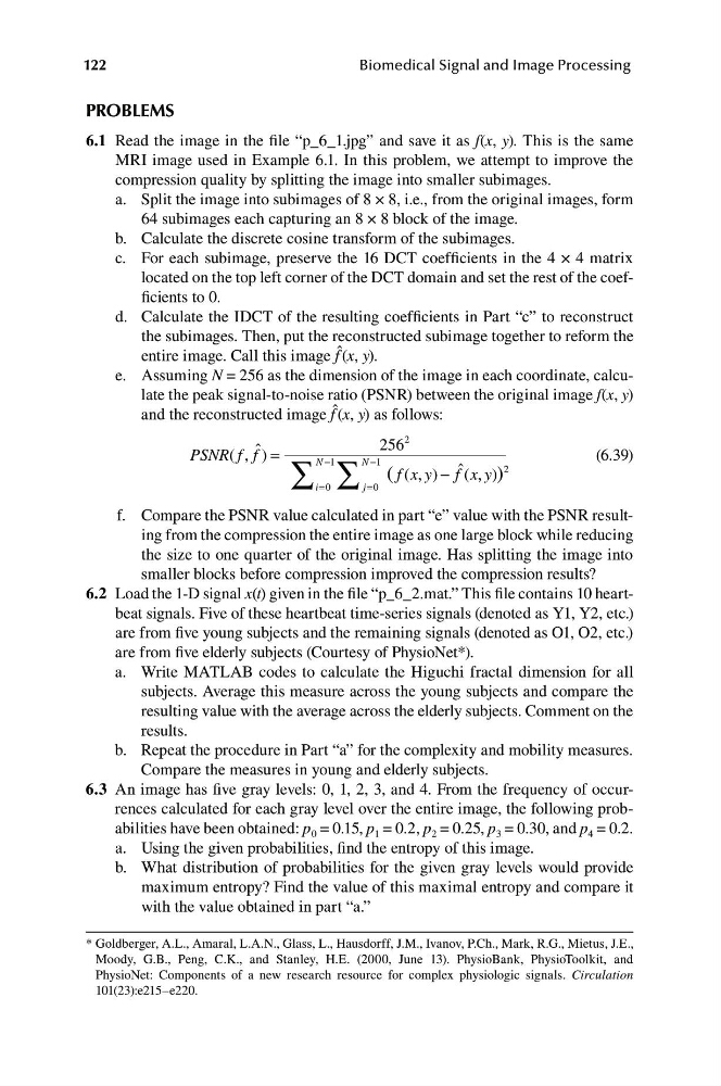
e. A ssuming N = 256 as the dimension of the image in each coordinate, calculate the peak signal-to-noise ratio (PSNR) between the original image f(x, y)
and the reconstructed image f ˆ (x, y) as follows:
256
2
ˆ
PSNR( ,
f f ) = ∑
N −1
∑
N −1
(6.39)
(
ˆ
f x
( , y ) − f (x, y ))
2
i=0
j =0
f. Compare the PSNR value calculated in part “e” value with the PSNR resulting from the compression the entire image as one large block while reducing
the size to one quarter of the original image. Has splitting the image into
smaller blocks before compression improved the compression results?
6.2 L oad the 1-D signal x(t) given in the file “p_6_2.mat.” This file contains 10 heartbeat signals. Five of these heartbeat time-series signals (denoted as Y1, Y2, etc.)
are from five young subjects and the remaining signals (denoted as O1, O2, etc.)
are from five elderly subjects (Courtesy of PhysioNet*).
a. W rite MATLAB codes to calculate the Higuchi fractal dimension for all
subjects. Average this measure across the young subjects and compare the
resulting value with the average across the elderly subjects. Comment on the
results.
b. R epeat the procedure in Part “a” for the complexity and mobility measures.
Compare the measures in young and elderly subjects.
6.3 An image has five gray levels: 0, 1, 2, 3, and 4. From the frequency of occurrences calculated for each gray level over the entire image, the following probabilities have been obtained: p 0 = 0.15, p 1 = 0.2, p 2 = 0.25, p 3 = 0.30, and p 4 = 0.2.
a. Using the given probabilities, find the entropy of this image.
b. W hat distribution of probabilities for the given gray levels would provide
maximum entropy? Find the value of this maximal entropy and compare it
with the value obtained in part “a.”
* Goldberger, A.L., Amaral, L.A.N., Glass, L., Hausdorff, J.M., Ivanov, P.Ch., Mark, R.G., Mietus, J.E.,
Moody, G.B., Peng, C.K., and Stanley, H.E. (2000, June 13). PhysioBank, PhysioToolkit, and
PhysioNet: Components of a new research resource for complex physiologic signals. Circulation
101(23):e215–e220.
Biomedical Signal and Image Processing
PROBLEMS
6.1 Read the image in the file “p_6_1.jpg” and save it as f(x, y). This is the same
MRI image used in Example 6.1. In this problem, we attempt to improve the
compression quality by splitting the image into smaller subimages.
a. S plit the image into subimages of 8 × 8, i.e., from the original images, form
64 subimages each capturing an 8 × 8 block of the image.
b. Calculate the discrete cosine transform of the subimages.
c. F or each subimage, preserve the 16 DCT coefficients in the 4 × 4 matrix
located on the top left corner of the DCT domain and set the rest of the coefficients to 0.
d. Ca lculate the IDCT of the resulting coefficients in Part “c” to reconstruct
the subimages. Then, put the reconstructed subimage together to reform the
entire image. Call this image f ˆ (x, y).
e. A ssuming N = 256 as the dimension of the image in each coordinate, calculate the peak signal-to-noise ratio (PSNR) between the original image f(x, y)
and the reconstructed image f ˆ (x, y) as follows:
256
2
ˆ
PSNR( ,
f f ) = ∑
N −1
∑
N −1
(6.39)
(
ˆ
f x
( , y ) − f (x, y ))
2
i=0
j =0
f. Compare the PSNR value calculated in part “e” value with the PSNR resulting from the compression the entire image as one large block while reducing
the size to one quarter of the original image. Has splitting the image into
smaller blocks before compression improved the compression results?
6.2 L oad the 1-D signal x(t) given in the file “p_6_2.mat.” This file contains 10 heartbeat signals. Five of these heartbeat time-series signals (denoted as Y1, Y2, etc.)
are from five young subjects and the remaining signals (denoted as O1, O2, etc.)
are from five elderly subjects (Courtesy of PhysioNet*).
a. W rite MATLAB codes to calculate the Higuchi fractal dimension for all
subjects. Average this measure across the young subjects and compare the
resulting value with the average across the elderly subjects. Comment on the
results.
b. R epeat the procedure in Part “a” for the complexity and mobility measures.
Compare the measures in young and elderly subjects.
6.3 An image has five gray levels: 0, 1, 2, 3, and 4. From the frequency of occurrences calculated for each gray level over the entire image, the following probabilities have been obtained: p 0 = 0.15, p 1 = 0.2, p 2 = 0.25, p 3 = 0.30, and p 4 = 0.2.
a. Using the given probabilities, find the entropy of this image.
b. W hat distribution of probabilities for the given gray levels would provide
maximum entropy? Find the value of this maximal entropy and compare it
with the value obtained in part “a.”
* Goldberger, A.L., Amaral, L.A.N., Glass, L., Hausdorff, J.M., Ivanov, P.Ch., Mark, R.G., Mietus, J.E.,
Moody, G.B., Peng, C.K., and Stanley, H.E. (2000, June 13). PhysioBank, PhysioToolkit, and
PhysioNet: Components of a new research resource for complex physiologic signals. Circulation
101(23):e215–e220.