

104
Biomedical Signal and Image Processing
for the wavelet-based measures is encouraged by the fact that in detecting specific
changes in a diseased signal (compared to normal signals), we need to know not only
the exact shape of these changes but also the length of the separation between the
changes (i.e., the scale of the change).
The wavelet measures commonly used in the biomedical studies are the wavelet
coefficients in high frequencies, which reflect the detailed high-frequency changes
across the signal. In order to better understand the use of high-frequency coefficients,
assume we are comparing two signals that are apparently similar to each other, for
example, a healthy and a diseased signal with high degree of similarities. The overall similarity of the two signals indicates that the wavelet coefficients describing
the overall approximation of the two signals are very similar (or the same). This
means that the wavelet coefficients in the low frequencies (i.e., large scales) are very
similar. But assuming that the two signals are indeed different, the wavelet theory
also asserts that the coefficients describing the details of the two signals must be different. This means that a comparison of the high-frequency (low-scale) coefficients
should reveal the differences of the two signals.
6.2.4 ENTROPY
Entropy is another measure of complexity, defined in information theory that is commonly used in biomedical signal and image processing. This measure is defined later
in this chapter when describing the fundamentals of coding and information theory.
6.3 COSINE TRANSFORM
In the previous chapters, we emphasized the importance of the techniques to compress a signal or an image. A popular technique for compression that is frequently
used in biomedical signal and image processing is cosine transform. Even though in
many compression applications, the cosine transform is being replaced by the wavelet
transform, we will briefly review this very useful technique. Since only discrete cosine
transform (DCT) is commonly used in real applications, we focus on the DCT. For
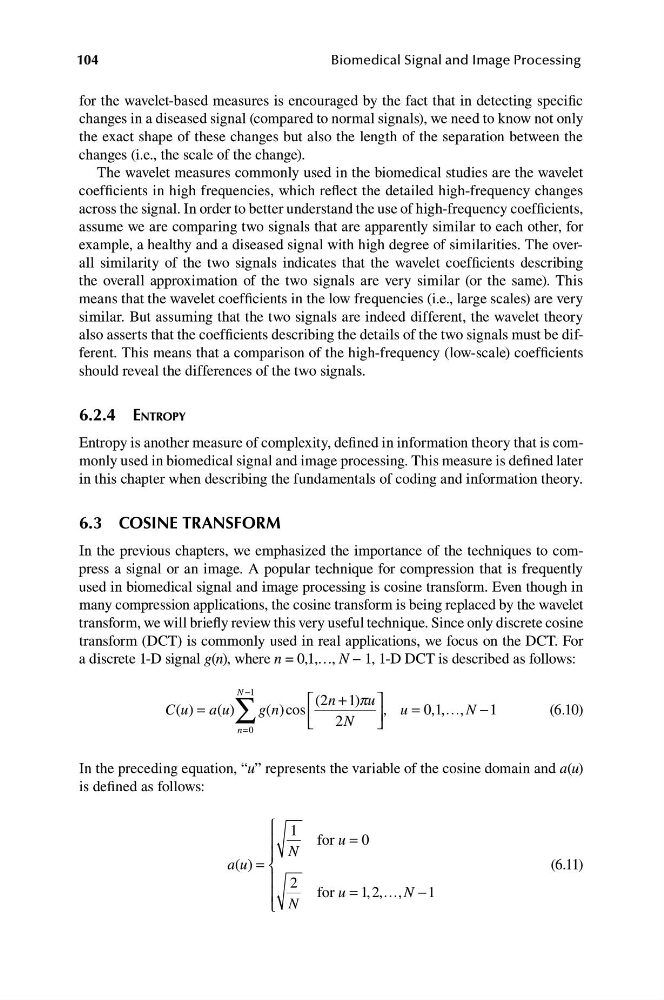
a discrete 1-D signal g(n), where n = 0,1,…, N − 1, 1-D DCT is described as follows:
∑
N −1
⎡ (2n + 1)pu ⎤
C u
( ) = a( )
u
g n
( )cos
, u = 0 1
, , …, N −
⎢
1
(6.10)
2N
⎥
n=0
⎣
⎦
In the preceding equation, “u” represents the variable of the cosine domain and a(u)
is defined as follows:
⎧ 1
⎪
for u = 0
⎪ N
a u
( ) = ⎨
(6.11)
⎪ 2
⎪
for u = 1 2
, ,…, N −1
⎩ N
Biomedical Signal and Image Processing
for the wavelet-based measures is encouraged by the fact that in detecting specific
changes in a diseased signal (compared to normal signals), we need to know not only
the exact shape of these changes but also the length of the separation between the
changes (i.e., the scale of the change).
The wavelet measures commonly used in the biomedical studies are the wavelet
coefficients in high frequencies, which reflect the detailed high-frequency changes
across the signal. In order to better understand the use of high-frequency coefficients,
assume we are comparing two signals that are apparently similar to each other, for
example, a healthy and a diseased signal with high degree of similarities. The overall similarity of the two signals indicates that the wavelet coefficients describing
the overall approximation of the two signals are very similar (or the same). This
means that the wavelet coefficients in the low frequencies (i.e., large scales) are very
similar. But assuming that the two signals are indeed different, the wavelet theory
also asserts that the coefficients describing the details of the two signals must be different. This means that a comparison of the high-frequency (low-scale) coefficients
should reveal the differences of the two signals.
6.2.4 ENTROPY
Entropy is another measure of complexity, defined in information theory that is commonly used in biomedical signal and image processing. This measure is defined later
in this chapter when describing the fundamentals of coding and information theory.
6.3 COSINE TRANSFORM
In the previous chapters, we emphasized the importance of the techniques to compress a signal or an image. A popular technique for compression that is frequently
used in biomedical signal and image processing is cosine transform. Even though in
many compression applications, the cosine transform is being replaced by the wavelet
transform, we will briefly review this very useful technique. Since only discrete cosine
transform (DCT) is commonly used in real applications, we focus on the DCT. For
a discrete 1-D signal g(n), where n = 0,1,…, N − 1, 1-D DCT is described as follows:
∑
N −1
⎡ (2n + 1)pu ⎤
C u
( ) = a( )
u
g n
( )cos
, u = 0 1
, , …, N −
⎢
1
(6.10)
2N
⎥
n=0
⎣
⎦
In the preceding equation, “u” represents the variable of the cosine domain and a(u)
is defined as follows:
⎧ 1
⎪
for u = 0
⎪ N
a u
( ) = ⎨
(6.11)
⎪ 2
⎪
for u = 1 2
, ,…, N −1
⎩ N