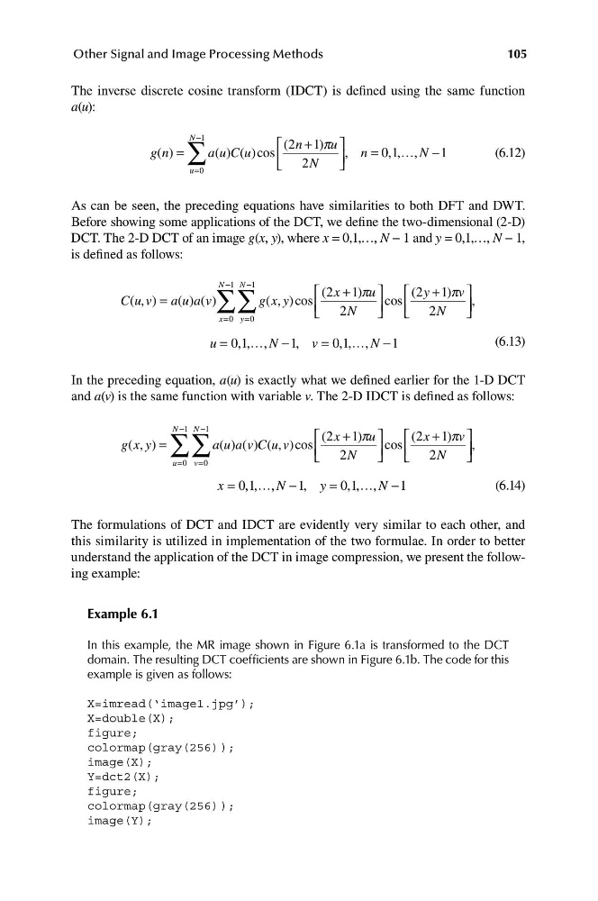
105
Other Signal and Image Processing Methods
The inverse discrete cosine transform (IDCT) is defined using the same function
a(u):
∑
N −1
⎡ (2n +1)pu ⎤
g n
( ) =
a( )
u C u
( )cos
= 0 1 …, N −
⎢ 2N
⎥ , n
, ,
1
(6.12)
u=0
⎣
⎦
As can be seen, the preceding equations have similarities to both DFT and DWT.
Before showing some applications of the DCT, we define the two-dimensional (2-D)
DCT. The 2-D DCT of an image g(x, y), where x = 0,1,…, N − 1 and y = 0,1,…, N − 1,
is defined as follows:
∑
N −1 ∑
N −1
⎡ (2x + 1)pu ⎤
⎡ (2y + 1)pv ⎤
C u
( ,v ) = a(u)a(v)
g(x, y ) cos ⎢
cos
,
2N
⎥
⎢ 2N
⎥ ⎥
x=0 y=0
⎣
⎦
⎣
⎦
u 0 1
, , , N 1 , v 0, ,
1 , N 1
(6.13)
=
… −
=
… −
In the preceding equation, a(u) is exactly what we defined earlier for the 1-D DCT
and a(v) is the same function with variable v. The 2-D IDCT is defined as follows:
∑
N −1 ∑
N −1
⎡ (2x + 1)pu ⎤
⎡ (2x + 1)pv ⎤
g x y
( , ) =
a(u) (
a v)C(u, v )cos ⎢
cos
,
⎣ 2N
⎥
⎢
⎦
N
⎥ ⎥
u=0 v=0
⎣ 2
⎦
x = 0 1
, , …, N −1 , y = 0, ,
1 …, N −1
(6.14)
The formulations of DCT and IDCT are evidently very similar to each other, and
this similarity is utilized in implementation of the two formulae. In order to better
understand the application of the DCT in image compression, we present the following example:
Example 6.1
In this example, the MR image shown in Figure 6.1a is transformed to the DCT
domain. The resulting DCT coefficients are shown in Figure 6.1b. The code for this
example is given as follows:
X=imread(‘image1.jpg’);

X=double(X);

figure;

colormap(gray(256) );

image(X);

Y=dct2(X);

figure;

colormap(gray(256) );

image(Y);