

1.3 Maxwell’s Equation
7
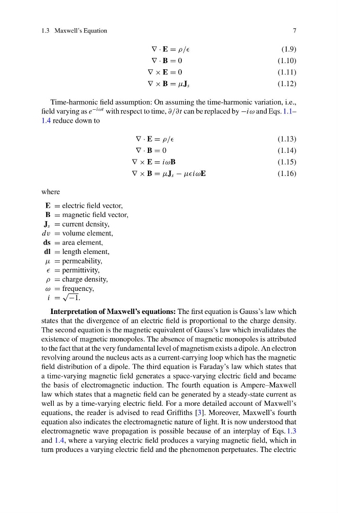
∇ · E = ρ//
(1.9)
∇ · B = 0
(1.10)
∇ × E = 0
(1.11)
∇ × B = μJ s
(1.12)
Time-harmonic field assumption: On assuming the time-harmonic variation, i.e.,
field varying as e
−iωt with respect to time, ∂/∂t can be replaced by −iω and Eqs. 1.1–
1.4 reduce down to
∇ · E = ρ//
(1.13)
∇ · B = 0
(1.14)
∇ × E = iωB
(1.15)
∇ × B = μJ s − μμiωE
(1.16)
where
E = electric field vector,
B = magnetic field vector,
J s = current density,
dv = volume element,
ds = area element,
dl = length element,
μ = permeability,
= permittivity,
ρ = charge density,
ω = frequency,
i =
√
−1.
Interpretation of Maxwell’s equations: The first equation is Gauss’s law which
states that the divergence of an electric field is proportional to the charge density.
The second equation is the magnetic equivalent of Gauss’s law which invalidates the
existence of magnetic monopoles. The absence of magnetic monopoles is attributed
to the fact that at the very fundamental level of magnetism exists a dipole. An electron
revolving around the nucleus acts as a current-carrying loop which has the magnetic
field distribution of a dipole. The third equation is Faraday’s law which states that
a time-varying magnetic field generates a space-varying electric field and became
the basis of electromagnetic induction. The fourth equation is Ampere–Maxwell
law which states that a magnetic field can be generated by a steady-state current as
well as by a time-varying electric field. For a more detailed account of Maxwell’s
equations, the reader is advised to read Griffiths [3]. Moreover, Maxwell’s fourth
equation also indicates the electromagnetic nature of light. It is now understood that
electromagnetic wave propagation is possible because of an interplay of Eqs. 1.3
and 1.4, where a varying electric field produces a varying magnetic field, which in
turn produces a varying electric field and the phenomenon perpetuates. The electric
7
∇ · E = ρ//
(1.9)
∇ · B = 0
(1.10)
∇ × E = 0
(1.11)
∇ × B = μJ s
(1.12)
Time-harmonic field assumption: On assuming the time-harmonic variation, i.e.,
field varying as e
−iωt with respect to time, ∂/∂t can be replaced by −iω and Eqs. 1.1–
1.4 reduce down to
∇ · E = ρ//
(1.13)
∇ · B = 0
(1.14)
∇ × E = iωB
(1.15)
∇ × B = μJ s − μμiωE
(1.16)
where
E = electric field vector,
B = magnetic field vector,
J s = current density,
dv = volume element,
ds = area element,
dl = length element,
μ = permeability,
= permittivity,
ρ = charge density,
ω = frequency,
i =
√
−1.
Interpretation of Maxwell’s equations: The first equation is Gauss’s law which
states that the divergence of an electric field is proportional to the charge density.
The second equation is the magnetic equivalent of Gauss’s law which invalidates the
existence of magnetic monopoles. The absence of magnetic monopoles is attributed
to the fact that at the very fundamental level of magnetism exists a dipole. An electron
revolving around the nucleus acts as a current-carrying loop which has the magnetic
field distribution of a dipole. The third equation is Faraday’s law which states that
a time-varying magnetic field generates a space-varying electric field and became
the basis of electromagnetic induction. The fourth equation is Ampere–Maxwell
law which states that a magnetic field can be generated by a steady-state current as
well as by a time-varying electric field. For a more detailed account of Maxwell’s
equations, the reader is advised to read Griffiths [3]. Moreover, Maxwell’s fourth
equation also indicates the electromagnetic nature of light. It is now understood that
electromagnetic wave propagation is possible because of an interplay of Eqs. 1.3
and 1.4, where a varying electric field produces a varying magnetic field, which in
turn produces a varying electric field and the phenomenon perpetuates. The electric