

5.4 Inventory Analysis (Phase 2)
77
Depending on the set system boundaries, this method can clearly reach its
practical limits quickly. To handle this, a calculation method using a linear system
of equations in the form of matrices has been developed.
5.4.4.2 Matrix Inversion Method
The matrix inversion method uses a system of linear equations to calculate the
cumulative resource uses and emissions of a system. This is done by setting up
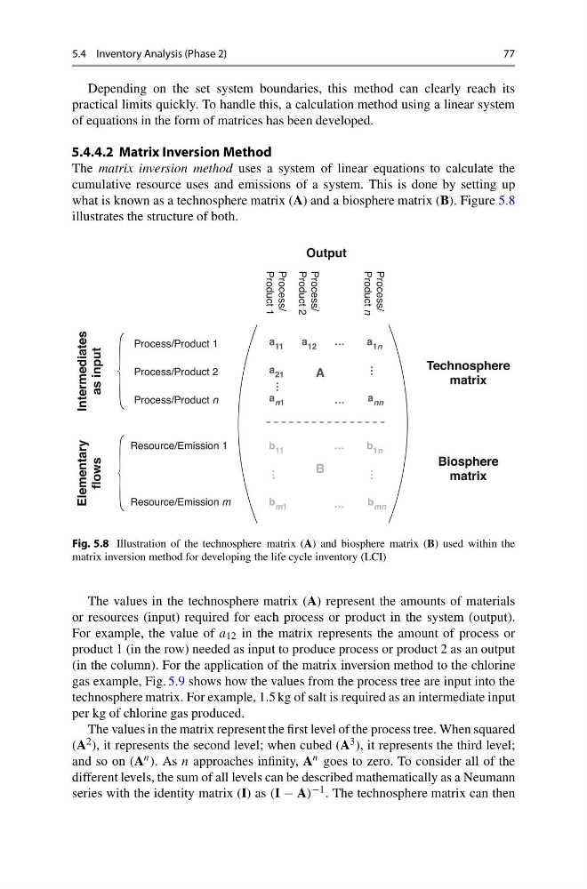
what is known as a technosphere matrix (A) and a biosphere matrix (B). Figure 5.8
illustrates the structure of both.
Fig. 5.8 Illustration of the technosphere matrix (A) and biosphere matrix (B) used within the
matrix inversion method for developing the life cycle inventory (LCI)
The values in the technosphere matrix (A) represent the amounts of materials
or resources (input) required for each process or product in the system (output).
For example, the value of a 12 in the matrix represents the amount of process or
product 1 (in the row) needed as input to produce process or product 2 as an output
(in the column). For the application of the matrix inversion method to the chlorine
gas example, Fig. 5.9 shows how the values from the process tree are input into the
technosphere matrix. For example, 1.5 kg of salt is required as an intermediate input
per kg of chlorine gas produced.
The values in the matrix represent the first level of the process tree. When squared
(A 2 ), it represents the second level; when cubed (A 3 ), it represents the third level;
and so on (A n ). As n approaches infinity, A n goes to zero. To consider all of the
different levels, the sum of all levels can be described mathematically as a Neumann
series with the identity matrix (I) as (I − A) −1 . The technosphere matrix can then
77
Depending on the set system boundaries, this method can clearly reach its
practical limits quickly. To handle this, a calculation method using a linear system
of equations in the form of matrices has been developed.
5.4.4.2 Matrix Inversion Method
The matrix inversion method uses a system of linear equations to calculate the
cumulative resource uses and emissions of a system. This is done by setting up
what is known as a technosphere matrix (A) and a biosphere matrix (B). Figure 5.8
illustrates the structure of both.
Fig. 5.8 Illustration of the technosphere matrix (A) and biosphere matrix (B) used within the
matrix inversion method for developing the life cycle inventory (LCI)
The values in the technosphere matrix (A) represent the amounts of materials
or resources (input) required for each process or product in the system (output).
For example, the value of a 12 in the matrix represents the amount of process or
product 1 (in the row) needed as input to produce process or product 2 as an output
(in the column). For the application of the matrix inversion method to the chlorine
gas example, Fig. 5.9 shows how the values from the process tree are input into the
technosphere matrix. For example, 1.5 kg of salt is required as an intermediate input
per kg of chlorine gas produced.
The values in the matrix represent the first level of the process tree. When squared
(A 2 ), it represents the second level; when cubed (A 3 ), it represents the third level;
and so on (A n ). As n approaches infinity, A n goes to zero. To consider all of the
different levels, the sum of all levels can be described mathematically as a Neumann
series with the identity matrix (I) as (I − A) −1 . The technosphere matrix can then