

282
D Dispersion Models
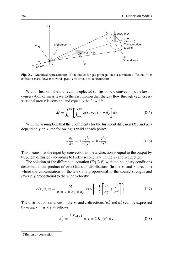
Fig. D.2 Graphical representation of the model for gas propagation via turbulent diffusion. ˙
M =
emission mass flow; u = wind speed; t = time; c = concentration
With diffusion in the x-direction neglected (diffusion << convection), the law of
conservation of mass leads to the assumption that the gas flow through each crosssectional area x is constant and equal to the flow ˙
M:
˙
M =
∞
0
∞
−∞
c(x, y, z) × u dy
dz
(D.5)
With the assumption that the coefficients for the turbulent diffusion (K y and K z )
depend only on x, the following is valid at each point:
u
∂c
∂x
= K y
∂ 2 c
∂y 2 + K z
∂ 2 c
∂z 2
(D.6)
This means that the input by convection in the x-direction is equal to the output by
turbulent diffusion (according to Fick’s second law) in the y- and z-direction.
The solution of the differential equation (Eq. D.6) with the boundary conditions
described is the product of two Gaussian distributions (in the y- and z-direction)
where the concentration on the x-axis is proportional to the source strength and
inversely proportional to the wind velocity: 1
c(x, y, z) =
˙
M
π × u × σ y × σ z
exp
−
1
2
y 2
σ 2
y
+
z 2
σ 2
z
(D.7)
The distribution variances in the y- and z-directions (σ 2
y and σ 2
y ) can be expressed
by using x = u × t as follows:
σ
2
y =
2 K y (x)
u
× x = 2 K y (x) × t
(D.8)
1 Dilution by convection
D Dispersion Models
Fig. D.2 Graphical representation of the model for gas propagation via turbulent diffusion. ˙
M =
emission mass flow; u = wind speed; t = time; c = concentration
With diffusion in the x-direction neglected (diffusion << convection), the law of
conservation of mass leads to the assumption that the gas flow through each crosssectional area x is constant and equal to the flow ˙
M:
˙
M =
∞
0
∞
−∞
c(x, y, z) × u dy
dz
(D.5)
With the assumption that the coefficients for the turbulent diffusion (K y and K z )
depend only on x, the following is valid at each point:
u
∂c
∂x
= K y
∂ 2 c
∂y 2 + K z
∂ 2 c
∂z 2
(D.6)
This means that the input by convection in the x-direction is equal to the output by
turbulent diffusion (according to Fick’s second law) in the y- and z-direction.
The solution of the differential equation (Eq. D.6) with the boundary conditions
described is the product of two Gaussian distributions (in the y- and z-direction)
where the concentration on the x-axis is proportional to the source strength and
inversely proportional to the wind velocity: 1
c(x, y, z) =
˙
M
π × u × σ y × σ z
exp
−
1
2
y 2
σ 2
y
+
z 2
σ 2
z
(D.7)
The distribution variances in the y- and z-directions (σ 2
y and σ 2
y ) can be expressed
by using x = u × t as follows:
σ
2
y =
2 K y (x)
u
× x = 2 K y (x) × t
(D.8)
1 Dilution by convection