

D.2 Gas Propagation by Turbulent Diffusion
281
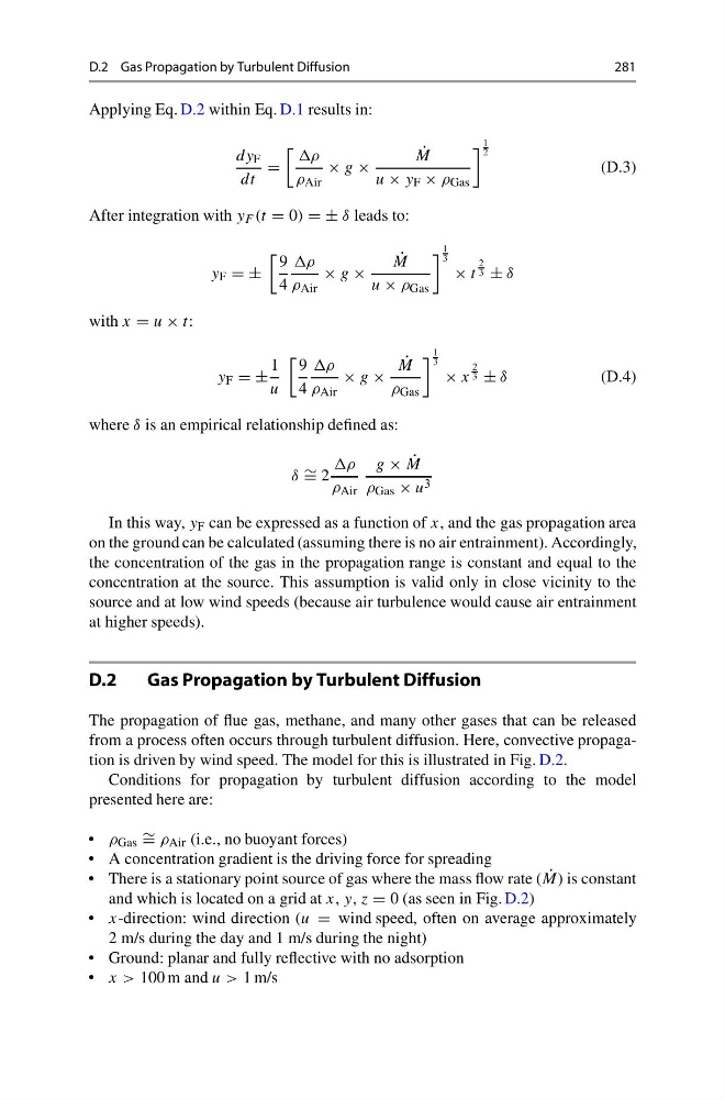
Applying Eq. D.2 within Eq. D.1 results in:
dy F
dt
=
ρ
ρ Air
× g ×
˙
M
u × y F × ρ Gas
1
2
(D.3)
After integration with y F (t = 0) = ± δ leads to:
y F = ±
9
4
ρ
ρ Air
× g ×
˙
M
u × ρ Gas
1
3
× t
2
3 ± δ
with x = u × t:
y F = ±
1
u
9
4
ρ
ρ Air
× g ×
˙
M
ρ Gas
1
3
× x
2
3 ± δ
(D.4)
where δ is an empirical relationship defined as:
δ ∼ = 2
ρ
ρ Air
g × ˙
M
ρ Gas × u 3
In this way, y F can be expressed as a function of x, and the gas propagation area
on the ground can be calculated (assuming there is no air entrainment). Accordingly,
the concentration of the gas in the propagation range is constant and equal to the
concentration at the source. This assumption is valid only in close vicinity to the
source and at low wind speeds (because air turbulence would cause air entrainment
at higher speeds).
D.2
Gas Propagation by Turbulent Diffusion
The propagation of flue gas, methane, and many other gases that can be released
from a process often occurs through turbulent diffusion. Here, convective propagation is driven by wind speed. The model for this is illustrated in Fig. D.2.
Conditions for propagation by turbulent diffusion according to the model
presented here are:
• ρ Gas ∼ = ρ Air (i.e., no buoyant forces)
• A concentration gradient is the driving force for spreading
• There is a stationary point source of gas where the mass flow rate ( ˙
M) is constant
and which is located on a grid at x, y, z = 0 (as seen in Fig. D.2)
• x-direction: wind direction (u = wind speed, often on average approximately
2 m/s during the day and 1 m/s during the night)
• Ground: planar and fully reflective with no adsorption
• x > 100 m and u > 1 m/s
281
Applying Eq. D.2 within Eq. D.1 results in:
dy F
dt
=
ρ
ρ Air
× g ×
˙
M
u × y F × ρ Gas
1
2
(D.3)
After integration with y F (t = 0) = ± δ leads to:
y F = ±
9
4
ρ
ρ Air
× g ×
˙
M
u × ρ Gas
1
3
× t
2
3 ± δ
with x = u × t:
y F = ±
1
u
9
4
ρ
ρ Air
× g ×
˙
M
ρ Gas
1
3
× x
2
3 ± δ
(D.4)
where δ is an empirical relationship defined as:
δ ∼ = 2
ρ
ρ Air
g × ˙
M
ρ Gas × u 3
In this way, y F can be expressed as a function of x, and the gas propagation area
on the ground can be calculated (assuming there is no air entrainment). Accordingly,
the concentration of the gas in the propagation range is constant and equal to the
concentration at the source. This assumption is valid only in close vicinity to the
source and at low wind speeds (because air turbulence would cause air entrainment
at higher speeds).
D.2
Gas Propagation by Turbulent Diffusion
The propagation of flue gas, methane, and many other gases that can be released
from a process often occurs through turbulent diffusion. Here, convective propagation is driven by wind speed. The model for this is illustrated in Fig. D.2.
Conditions for propagation by turbulent diffusion according to the model
presented here are:
• ρ Gas ∼ = ρ Air (i.e., no buoyant forces)
• A concentration gradient is the driving force for spreading
• There is a stationary point source of gas where the mass flow rate ( ˙
M) is constant
and which is located on a grid at x, y, z = 0 (as seen in Fig. D.2)
• x-direction: wind direction (u = wind speed, often on average approximately
2 m/s during the day and 1 m/s during the night)
• Ground: planar and fully reflective with no adsorption
• x > 100 m and u > 1 m/s