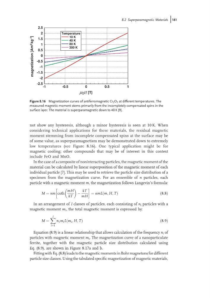
not show any hysteresis, although a minor hysteresis is seen at 10 K. When
considering technical applications for these materials, the residual magnetic
moment stemming from incomplete compensated spins at the surface may be
of some value, as superparamagnetism may be demonstrated down to extremely
low temperatures (see Figure 8.16). One typical application might be for
magnetic cooling; other compounds that may be of interest in this context
include FeO and MnO.
In the case of a composite of noninteracting particles, the magnetic moment of the
material can be calculated by linear superposition of the magnetic moment of each
individual particle [7]. This may be used to retrieve the particle size distribution of a
specimen from the magnetization curve. For an ensemble of n particles, each
particle with a magnetic moment m, the magnetization follows Langevin’s formula:
M ¼ nm coth
mH
kT
À
kT
mH
¼ nmL m; H; T
ð
Þ
ð 8:8Þ
In an arrangement of I classes of particles, each consisting of n i particles with a
magnetic moment m i , the total magnetic moment is expressed by:
M ¼
X I
i¼1
n 1 m i Lðm i ; H; TÞ
ð 8:9Þ
Equation (8.9) is a linear relationship that allows calculation of the frequency n i of
particles with magnetic moment m i . The magnetization curve of a nanoparticulate
ferrite, together with the magnetic particle size distribution calculated using
Eq. (8.9), are shown in Figure 8.17a and b.
Fitting with Eq. (8.8) leads to the magnetic moments in Bohr magnetons for different
particle size classes. Using the tabulated specific magnetization of magnetic materials,
-1
-0.5
0
0.5
1
μ 0 H [T]
-2.5
-2
-1.5
-1
-0.5
0
0.5
1
1.5
2
2.5
magnetization
[Am
2 -1
kg
]
Temperature
10 K
40 K
80 K
300 K
Figure 8.16 Magnetization curves of antiferromagnetic Cr 2 O 3 at different temperatures. The
measured magnetic moment stems primarily from the incompletely compensated spins in the
surface layer. The material is superparamagnetic down to 40 K [9].
8.2 Superparamagnetic Materials j181