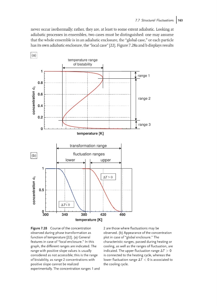
never occur isothermally; rather, they are, at least to some extent adiabatic. Looking at
adiabatic processes in ensembles, two cases must be distinguished: one may assume
that the whole ensemble is in an adiabatic enclosure, the “global case,” or each particle
has its own adiabatic enclosure, the “local case” [22]. Figure 7.28a and b displays results
0
0.2
0.4
0.6
0.8
1
concentration
c 1
temperature range
(a)
of bistability
1
range
2
range
3
range
temperature [K]
300
340
380
420
460
temperature [K]
0
0.5
1
concentration
c 1
⎯ T< 0
ΔT > 0
fluctuation ranges
upper
lower
transformation range
Δ
(b)
Figure 7.28 Course of the concentration
observed during phase transformation as
function of temperature [22]. (a) General
features in case of “local enclosure.” In this
graph, the different ranges are indicated. The
range with positive slope values is usually
considered as not accessible; this is the range
of bistability, as range 2 concentrations with
positive slope cannot be realized
experimentally. The concentration ranges 1 and
2 are those where fluctuations may be
observed. (b) Appearance of the concentration
plot in case of “global enclosure.” The
characteristic ranges, passed during heating or
cooling, as well as the ranges of fluctuation, are
indicated. The upper fluctuation range DT > 0
is connected to the heating cycle, whereas the
lower fluctuation range DT < 0 is associated to
the cooling cycle.
7.7 Structural Fluctuations j163