

zero, the fluctuations characterize the system. Therefore, Eq. (7.18) reflects the wellknown fact that besides geometry, fluctuations are ruled only by the entropy of
transformation DS trans ; d also has the dimension of entropy.
A phase diagram designed by using Eqs. (7.9) and (7.12) resembles those
calculated by Ajayan and Marks [20] for the phase limits of the quasimelt. However,
when examining the experimental results reported by Oshima and Takayanagi [21],
it is possible that these equations do not describe the experimental findings. One
reason for this discrepancy might be that the denominator in Eq. (7.18) is not
constant, and indeed both experimental indications and theoretical results [18] have
shown that the thermodynamic quantities DU trans and DS trans are particle sizedependent. This is necessary because it has been well documented experimentally –
and backed up by theory – that small particles, notably those less than 5 nm, show an
inherently high degree of disorder which increases with decreasing particle size.
In general, one never analyzes the behavior of a single particle, but rather that of a
system of many particles, termed an ensemble. Here, the use of a central theorem of
statistical thermodynamics – the ergodic theorem – simplifies the task. (According
to Boltzmann and Gibbs, in an ergodic system a time average can be replaced by an
ensemble average, when phase transformation occurs from one level (old phase) to a
second level (new phase). In a simplified way, this says that there is no difference if
one performs an experiment n times with one particle or one time with n particles.)
The probabilities of the relative time periods can then be measured either with one
particle in two different phases, or with an ensemble of particles, the numbers of
which can be counted in each phase.
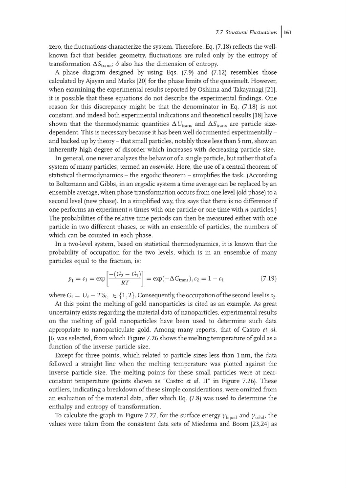
In a two-level system, based on statistical thermodynamics, it is known that the
probability of occupation for the two levels, which is in an ensemble of many
particles equal to the fraction, is:
p 1 ¼ c 1 ¼ exp
À G 2 À G 1
ð
Þ
RT
¼ exp ÀDG trans
ð
Þ ; c 2 ¼ 1 À c 1
ð7:19Þ
where G i ¼ U i À TS i ; 2 1; 2
f g. Consequently, the occupation of the second level is c 2 .
At this point the melting of gold nanoparticles is cited as an example. As great
uncertainty exists regarding the material data of nanoparticles, experimental results
on the melting of gold nanoparticles have been used to determine such data
appropriate to nanoparticulate gold. Among many reports, that of Castro et al.
[6] was selected, from which Figure 7.26 shows the melting temperature of gold as a
function of the inverse particle size.
Except for three points, which related to particle sizes less than 1 nm, the data
followed a straight line when the melting temperature was plotted against the
inverse particle size. The melting points for these small particles were at nearconstant temperature (points shown as “Castro et al. II” in Figure 7.26). These
outliers, indicating a breakdown of these simple considerations, were omitted from
an evaluation of the material data, after which Eq. (7.8) was used to determine the
enthalpy and entropy of transformation.
To calculate the graph in Figure 7.27, for the surface energy c liquid and c solid , the
values were taken from the consistent data sets of Miedema and Boom [23,24] as
7.7 Structural Fluctuations j161
transformation DS trans ; d also has the dimension of entropy.
A phase diagram designed by using Eqs. (7.9) and (7.12) resembles those
calculated by Ajayan and Marks [20] for the phase limits of the quasimelt. However,
when examining the experimental results reported by Oshima and Takayanagi [21],
it is possible that these equations do not describe the experimental findings. One
reason for this discrepancy might be that the denominator in Eq. (7.18) is not
constant, and indeed both experimental indications and theoretical results [18] have
shown that the thermodynamic quantities DU trans and DS trans are particle sizedependent. This is necessary because it has been well documented experimentally –
and backed up by theory – that small particles, notably those less than 5 nm, show an
inherently high degree of disorder which increases with decreasing particle size.
In general, one never analyzes the behavior of a single particle, but rather that of a
system of many particles, termed an ensemble. Here, the use of a central theorem of
statistical thermodynamics – the ergodic theorem – simplifies the task. (According
to Boltzmann and Gibbs, in an ergodic system a time average can be replaced by an
ensemble average, when phase transformation occurs from one level (old phase) to a
second level (new phase). In a simplified way, this says that there is no difference if
one performs an experiment n times with one particle or one time with n particles.)
The probabilities of the relative time periods can then be measured either with one
particle in two different phases, or with an ensemble of particles, the numbers of
which can be counted in each phase.
In a two-level system, based on statistical thermodynamics, it is known that the
probability of occupation for the two levels, which is in an ensemble of many
particles equal to the fraction, is:
p 1 ¼ c 1 ¼ exp
À G 2 À G 1
ð
Þ
RT
¼ exp ÀDG trans
ð
Þ ; c 2 ¼ 1 À c 1
ð7:19Þ
where G i ¼ U i À TS i ; 2 1; 2
f g. Consequently, the occupation of the second level is c 2 .
At this point the melting of gold nanoparticles is cited as an example. As great
uncertainty exists regarding the material data of nanoparticles, experimental results
on the melting of gold nanoparticles have been used to determine such data
appropriate to nanoparticulate gold. Among many reports, that of Castro et al.
[6] was selected, from which Figure 7.26 shows the melting temperature of gold as a
function of the inverse particle size.
Except for three points, which related to particle sizes less than 1 nm, the data
followed a straight line when the melting temperature was plotted against the
inverse particle size. The melting points for these small particles were at nearconstant temperature (points shown as “Castro et al. II” in Figure 7.26). These
outliers, indicating a breakdown of these simple considerations, were omitted from
an evaluation of the material data, after which Eq. (7.8) was used to determine the
enthalpy and entropy of transformation.
To calculate the graph in Figure 7.27, for the surface energy c liquid and c solid , the
values were taken from the consistent data sets of Miedema and Boom [23,24] as
7.7 Structural Fluctuations j161