

d ¼
ffiffi ffi
3
p
p
a CÀC n
2 þ m
2 þ nm
À
Á 0:5 ¼ 0:0783 n
2 þ m
2 þ nm
À
Á 0:5 nm
½
ð5:6Þ
where a CÀC ¼ 0:14 nm is the distance between two neighboring carbon atoms. In
reality, the range of diameters of carbon nanotubes is limited. Experimentally,
single-wall carbon nanotubes are observed with diameters ranging from 1.2 to
1.4 nm. However, nanotubes with significant larger diameters may also be produced. The chiral angle (i.e., the angle between the~ e 1 axis and the chirality vector~ c)
is given by:
d ¼ arctan
ffiffi ffi
3
p
3
2n þ m
!
ð5:7Þ
The chiral angle for the armchair line is 30
and that for the zig-zag line is 0
. Carbon
nanotubes with a chirality vector fulfilling the condition q ¼ ð2n þ mÞ=3; q 2 N,
show metallic electrical conductivity. In Figure 5.17, these vertices are indicated with
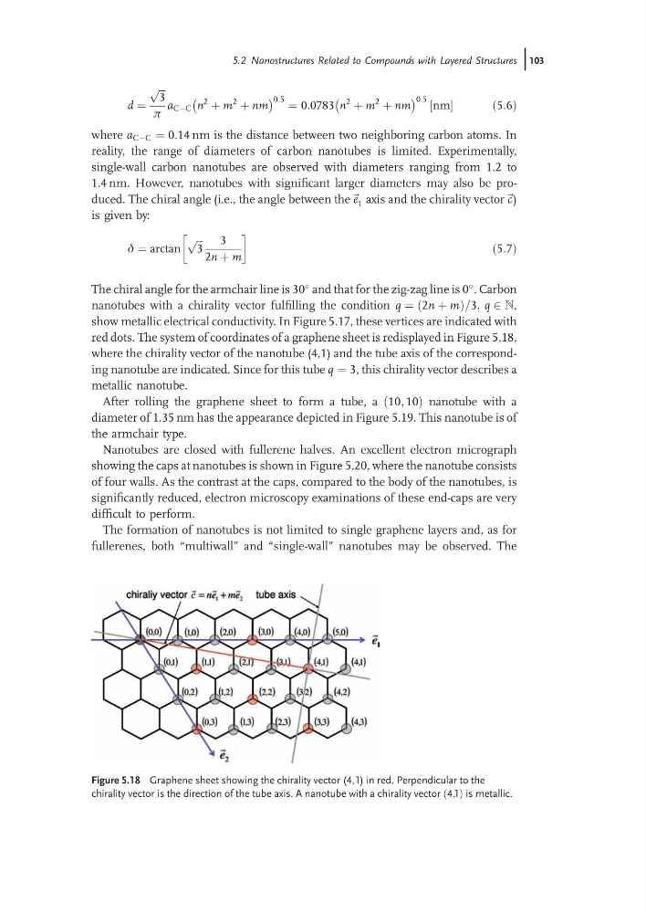
red dots. The system of coordinates of a graphene sheet is redisplayed in Figure 5.18,
where the chirality vector of the nanotube (4,1) and the tube axis of the corresponding nanotube are indicated. Since for this tube q ¼ 3, this chirality vector describes a
metallic nanotube.
After rolling the graphene sheet to form a tube, a 10; 10
ð
Þ nanotube with a
diameter of 1.35 nm has the appearance depicted in Figure 5.19. This nanotube is of
the armchair type.
Nanotubes are closed with fullerene halves. An excellent electron micrograph
showing the caps at nanotubes is shown in Figure 5.20, where the nanotube consists
of four walls. As the contrast at the caps, compared to the body of the nanotubes, is
significantly reduced, electron microscopy examinations of these end-caps are very
difficult to perform.
The formation of nanotubes is not limited to single graphene layers and, as for
fullerenes, both “multiwall” and “single-wall” nanotubes may be observed. The
Figure 5.18 Graphene sheet showing the chirality vector (4,1) in red. Perpendicular to the
chirality vector is the direction of the tube axis. A nanotube with a chirality vector 4; 1
ð Þis metallic.
5.2 Nanostructures Related to Compounds with Layered Structures j103
ffiffi ffi
3
p
p
a CÀC n
2 þ m
2 þ nm
À
Á 0:5 ¼ 0:0783 n
2 þ m
2 þ nm
À
Á 0:5 nm
½
ð5:6Þ
where a CÀC ¼ 0:14 nm is the distance between two neighboring carbon atoms. In
reality, the range of diameters of carbon nanotubes is limited. Experimentally,
single-wall carbon nanotubes are observed with diameters ranging from 1.2 to
1.4 nm. However, nanotubes with significant larger diameters may also be produced. The chiral angle (i.e., the angle between the~ e 1 axis and the chirality vector~ c)
is given by:
d ¼ arctan
ffiffi ffi
3
p
3
2n þ m
!
ð5:7Þ
The chiral angle for the armchair line is 30
and that for the zig-zag line is 0
. Carbon
nanotubes with a chirality vector fulfilling the condition q ¼ ð2n þ mÞ=3; q 2 N,
show metallic electrical conductivity. In Figure 5.17, these vertices are indicated with
red dots. The system of coordinates of a graphene sheet is redisplayed in Figure 5.18,
where the chirality vector of the nanotube (4,1) and the tube axis of the corresponding nanotube are indicated. Since for this tube q ¼ 3, this chirality vector describes a
metallic nanotube.
After rolling the graphene sheet to form a tube, a 10; 10
ð
Þ nanotube with a
diameter of 1.35 nm has the appearance depicted in Figure 5.19. This nanotube is of
the armchair type.
Nanotubes are closed with fullerene halves. An excellent electron micrograph
showing the caps at nanotubes is shown in Figure 5.20, where the nanotube consists
of four walls. As the contrast at the caps, compared to the body of the nanotubes, is
significantly reduced, electron microscopy examinations of these end-caps are very
difficult to perform.
The formation of nanotubes is not limited to single graphene layers and, as for
fullerenes, both “multiwall” and “single-wall” nanotubes may be observed. The
Figure 5.18 Graphene sheet showing the chirality vector (4,1) in red. Perpendicular to the
chirality vector is the direction of the tube axis. A nanotube with a chirality vector 4; 1
ð Þis metallic.
5.2 Nanostructures Related to Compounds with Layered Structures j103