

The convolution layer extracts different levels of features from the input image to
obtain feature maps. The model passes the output of the last convolutional layer to the
three fully connected layers, ultimately resulting in the position of the predicted
bounding box cx; cy; w; h. Where cx, cy is the center point x coordinate of the bounding
box, the center point y coordinate, w, h are the width and height, respectively.
The detection model input an image and predicts the bounding box of the LP
position in the image. The localization loss (see Eq. 2.1) is a Smooth L1 loss between
the predicted box (pb) and the ground truth box (gb). Where N is the batch size in
training, pb
m is one of the four coordinates cx, cy, w, h of the predicted bounding box,
gb
m is one of the four coordinates cx, cy, w, h of the ground truth bounding box. The
parameters were updated using a stochastic gradient descent (SGD) method.
Loss pb, gb
ð
Þ¼
X
N
X
m2 cx;cy;w;h
f
g
smooth L1 pb
m
À gb
m
ð
Þ
ð 2:1Þ
3 Visualization with a DeconvNet
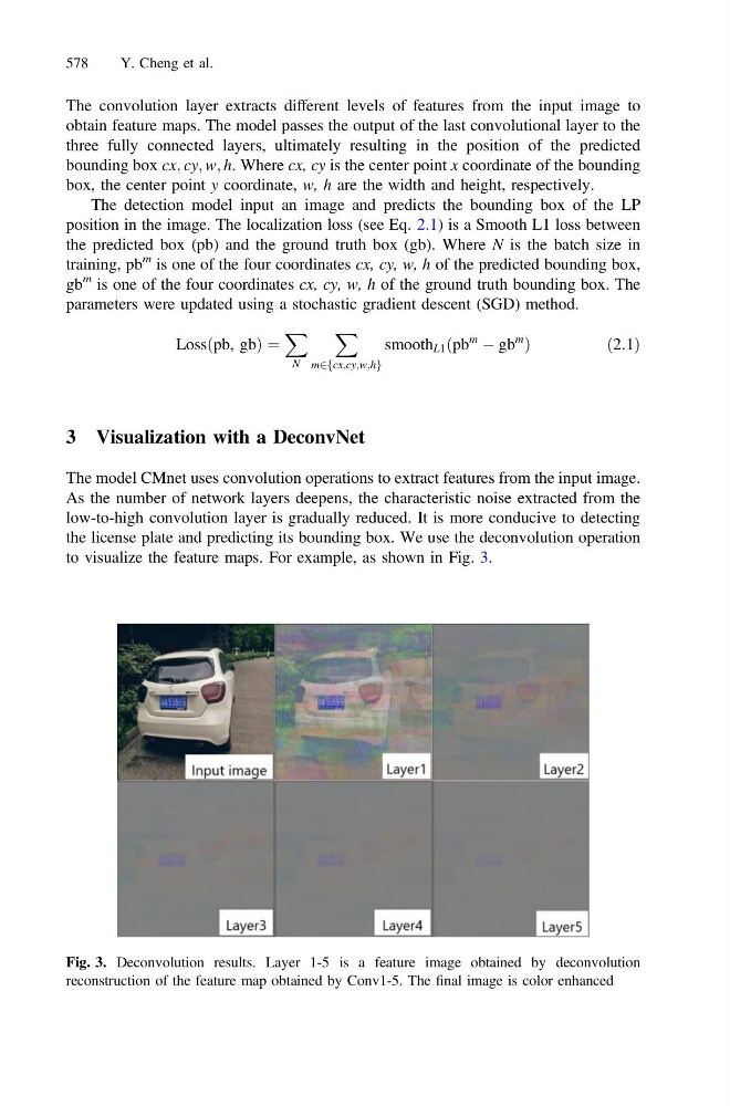
The model CMnet uses convolution operations to extract features from the input image.
As the number of network layers deepens, the characteristic noise extracted from the
low-to-high convolution layer is gradually reduced. It is more conducive to detecting
the license plate and predicting its bounding box. We use the deconvolution operation
to visualize the feature maps. For example, as shown in Fig. 3.
Fig. 3. Deconvolution results. Layer 1-5 is a feature image obtained by deconvolution
reconstruction of the feature map obtained by Conv1-5. The final image is color enhanced
578
Y. Cheng et al.