L f
ð Þ ¼ logðAðf ÞÞ:
ð8Þ
R f
ð Þ ¼ Lðf Þ À h m f
ð Þ Ã Lðf Þ:
ð9Þ
where h m represents the mean filtered convolution kernel, which is expressed as
h m ¼
1
9
1 1 1
1 1 1
1 1 1
2
4
3
5 :
ð10Þ
In order to obtain a better visual effect, the Gaussian kernel g(x) is used to smooth
the saliency map, and the obtained image saliency score is shown in Eq. (11), where
the inverse Fourier transform is shown.
SalS x
ð Þ ¼ g x
ð Þ Ã F
À1 exp R f
ð Þ þ P f
ð Þ
ð
Þ
ð
Þ
2 :
ð11Þ
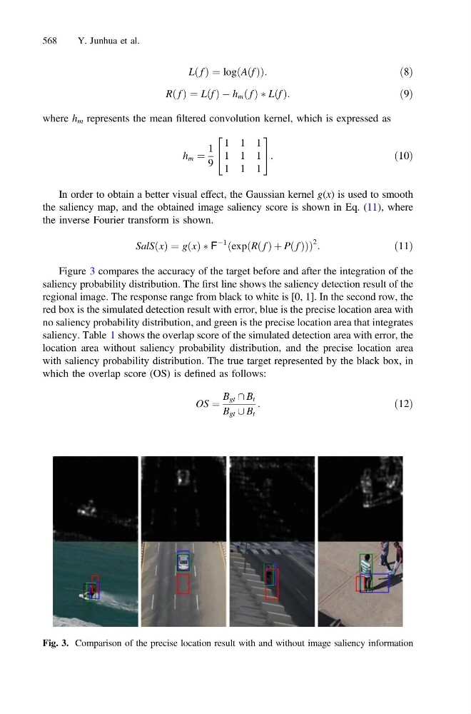
Figure 3 compares the accuracy of the target before and after the integration of the
saliency probability distribution. The first line shows the saliency detection result of the
regional image. The response range from black to white is [0, 1]. In the second row, the
red box is the simulated detection result with error, blue is the precise location area with
no saliency probability distribution, and green is the precise location area that integrates
saliency. Table 1 shows the overlap score of the simulated detection area with error, the
location area without saliency probability distribution, and the precise location area
with saliency probability distribution. The true target represented by the black box, in
which the overlap score (OS) is defined as follows:
OS ¼
B gt \ B t
B gt [ B t
:
ð12Þ
Fig. 3. Comparison of the precise location result with and without image saliency information
568
Y. Junhua et al.