

540
M. Ma et al.
where x
t is the estimate of the true signal at iteration t and z
t is an estimate
of the residual. x
t + A ∗ z
t can be considered as i.i.d. Gaussian noise. ˆ
σ
t is an
estimate of the standard deviation of the noise. div D ˆ
σ t−1 denotes the divergence
of the denoiser.
Each iteration of the D-AMP algorithm can be regarded as a denoising operation, so the performance of the denoiser directly affects the final reconstruction
result.
3.2 Typical Denoiser and Their Results
The image denoising model can be expressed as the following optimization problem:
arg min
ˆ
x
− ˆ
x
2
2 ,
(3)
where z is the noise image, x is the true image. The goal of the denoiser is to
find the closest estimate ˆ
x to x.
There are three main streams in up-to-date image denoisers, here we introduce one typical denoiser for each.
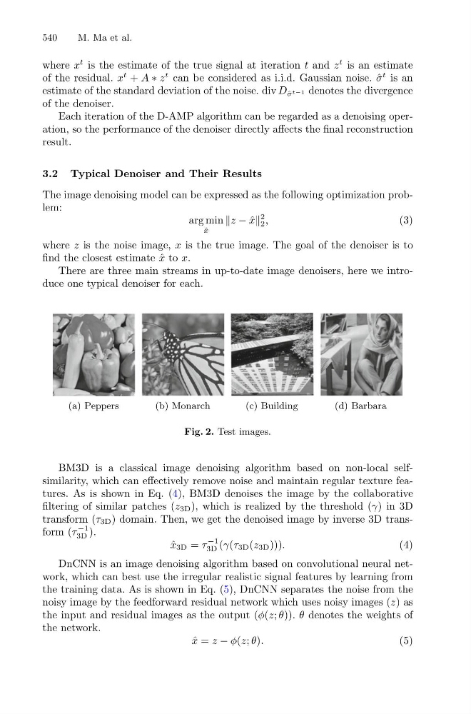
(a) Peppers
(b) Monarch
(c) Building
(d) Barbara
Fig. 2. Test images.
BM3D is a classical image denoising algorithm based on non-local selfsimilarity, which can effectively remove noise and maintain regular texture features. As is shown in Eq. (4), BM3D denoises the image by the collaborative
filtering of similar patches (z 3D ), which is realized by the threshold (γ) in 3D
transform (τ 3D ) domain. Then, we get the denoised image by inverse 3D transform (τ
−1
3D ).
ˆ
x 3D = τ
−1
3D (γ(τ 3D (z 3D ))).
(4)
DnCNN is an image denoising algorithm based on convolutional neural network, which can best use the irregular realistic signal features by learning from
the training data. As is shown in Eq. (5), DnCNN separates the noise from the
noisy image by the feedforward residual network which uses noisy images (z) as
the input and residual images as the output (φ(z; θ)). θ denotes the weights of
the network.
ˆ
x = z − φ(z; θ).
(5)