

3 Simulation
All simulations are based on the half-wavelength separation uniform linear array.
Considering the carry frequency will not affect the results, we take zero-carried frequency LFM signal as sðtÞ ¼ e
jpK r t
2 , whose frequency modulation rate is K r ¼ B=s,
and the time is Às=2 t s=2. The false-alarm rate is set as p f ¼ 0:01.
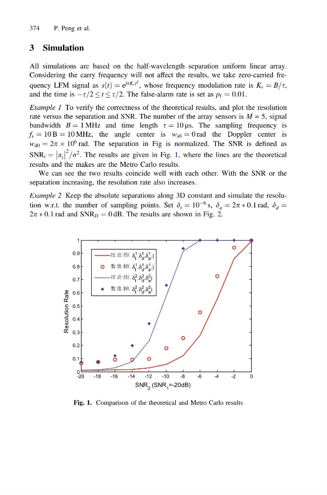
Example 1 To verify the correctness of the theoretical results, and plot the resolution
rate versus the separation and SNR. The number of the array sensors is M = 5, signal
bandwidth B ¼ 1 MHz and time length s ¼ 10 ls. The sampling frequency is
f s ¼ 10 B ¼ 10 MHz, the angle center is w s0 ¼ 0 rad the Doppler center is
w d0 ¼ 2p  10
6 rad. The separation in Fig is normalized. The SNR is defined as
SNR i ¼ a i
2 =r
2 . The results are given in Fig. 1, where the lines are the theoretical
results and the makes are the Metro Carlo results.
We can see the two results coincide well with each other. With the SNR or the
separation increasing, the resolution rate also increases.
Example 2 Keep the absolute separations along 3D constant and simulate the resolution w.r.t. the number of sampling points. Set d t ¼ 10
À6 s, d a ¼ 2p à 0:1 rad, d d ¼
2p à 0:1 rad and SNR D ¼ 0 dB. The results are shown in Fig. 2.
-20
-18
-16
-14
-12
-10
-8
-6
-4
-2
0
0
0.1
0.2
0.3
0.4
0.5
0.6
0.7
0.8
0.9
1
SNR 2 (SNR 1 =-20dB)
Resolution Rate
δ t
1
,δ d
1
,δ a
1
,)
δ t
1
,δ d
1
,δ a
1
,)
δ t
2
,δ d
2
,δ a
2
)
δ t
2
,δ d
2
,δ a
2
)
Fig. 1. Comparison of the theoretical and Metro Carlo results
374
P. Peng et al.
All simulations are based on the half-wavelength separation uniform linear array.
Considering the carry frequency will not affect the results, we take zero-carried frequency LFM signal as sðtÞ ¼ e
jpK r t
2 , whose frequency modulation rate is K r ¼ B=s,
and the time is Às=2 t s=2. The false-alarm rate is set as p f ¼ 0:01.
Example 1 To verify the correctness of the theoretical results, and plot the resolution
rate versus the separation and SNR. The number of the array sensors is M = 5, signal
bandwidth B ¼ 1 MHz and time length s ¼ 10 ls. The sampling frequency is
f s ¼ 10 B ¼ 10 MHz, the angle center is w s0 ¼ 0 rad the Doppler center is
w d0 ¼ 2p  10
6 rad. The separation in Fig is normalized. The SNR is defined as
SNR i ¼ a i
2 =r
2 . The results are given in Fig. 1, where the lines are the theoretical
results and the makes are the Metro Carlo results.
We can see the two results coincide well with each other. With the SNR or the
separation increasing, the resolution rate also increases.
Example 2 Keep the absolute separations along 3D constant and simulate the resolution w.r.t. the number of sampling points. Set d t ¼ 10
À6 s, d a ¼ 2p à 0:1 rad, d d ¼
2p à 0:1 rad and SNR D ¼ 0 dB. The results are shown in Fig. 2.
-20
-18
-16
-14
-12
-10
-8
-6
-4
-2
0
0
0.1
0.2
0.3
0.4
0.5
0.6
0.7
0.8
0.9
1
SNR 2 (SNR 1 =-20dB)
Resolution Rate
δ t
1
,δ d
1
,δ a
1
,)
δ t
1
,δ d
1
,δ a
1
,)
δ t
2
,δ d
2
,δ a
2
)
δ t
2
,δ d
2
,δ a
2
)
Fig. 1. Comparison of the theoretical and Metro Carlo results
374
P. Peng et al.