

1.2 3D Resolution Statistical and Its Performance
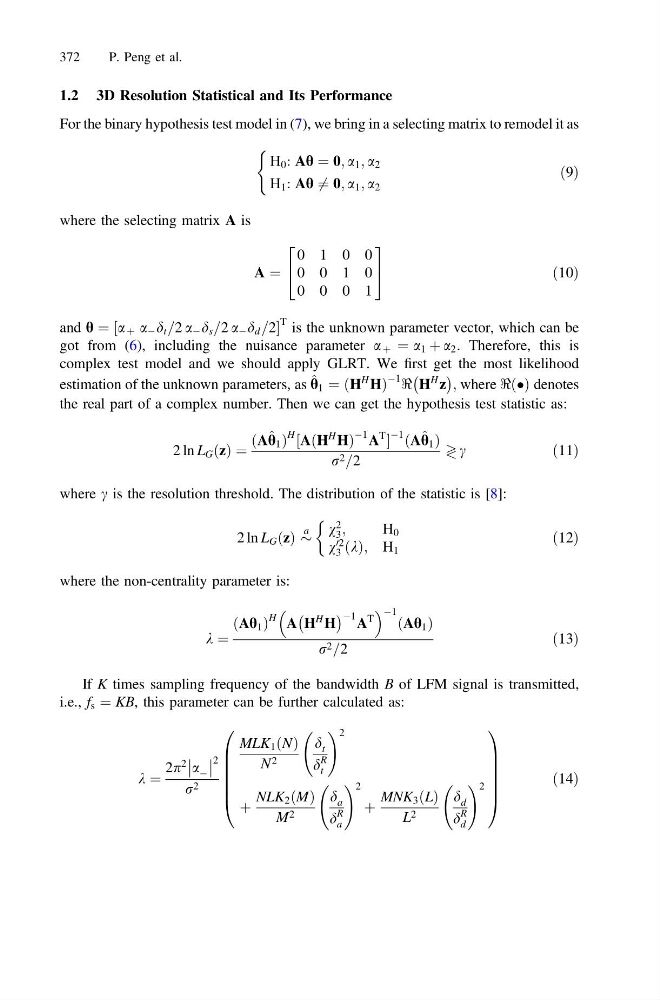
For the binary hypothesis test model in (7), we bring in a selecting matrix to remodel it as
H 0 : Ah ¼ 0; a 1 ; a 2
H 1 : Ah 6 ¼ 0; a 1 ; a 2
(
ð9Þ
where the selecting matrix A is
A ¼
0 1 0 0
0 0 1 0
0 0 0 1
2
4
3
5
ð10Þ
and h ¼ a þ a À d t =2 a À d s =2 a À d d =2
½
T is the unknown parameter vector, which can be
got from (6), including the nuisance parameter a þ ¼ a 1 þ a 2 . Therefore, this is
complex test model and we should apply GLRT. We first get the most likelihood
estimation of the unknown parameters, as ^ h 1 ¼ ðH
H HÞ
À1 < H
H z
À
Á ; where <ðÞ denotes
the real part of a complex number. Then we can get the hypothesis test statistic as:
2 ln L G ðzÞ ¼
ðA ^ h 1 Þ
H ½AðH
H HÞ
À1 A
T
À1 ðA ^ h 1 Þ
r 2 =2
? c
ð11Þ
where c is the resolution threshold. The distribution of the statistic is [8]:
2 ln L G ðzÞ $
a
v
2
3 ;
H 0
v
02
3 ðkÞ; H 1
&
ð12Þ
where the non-centrality parameter is:
k ¼
Ah 1
ð
Þ
H A H
H H
À
Á À1 A
T
À1
Ah 1
ð
Þ
r 2 =2
ð13Þ
If K times sampling frequency of the bandwidth B of LFM signal is transmitted,
i.e., f s ¼ KB, this parameter can be further calculated as:
k ¼
2p
2
a À
2
r 2
MLK 1 ðNÞ
N 2
d t
d
R
t
! 2
þ
NLK 2 ðMÞ
M 2
d a
d
R
a
! 2
þ
MNK 3 ðLÞ
L 2
d d
d
R
d
! 2
0
B
B
B
B
B
@
1
C
C
C
C
C
A
ð14Þ
372
P. Peng et al.
For the binary hypothesis test model in (7), we bring in a selecting matrix to remodel it as
H 0 : Ah ¼ 0; a 1 ; a 2
H 1 : Ah 6 ¼ 0; a 1 ; a 2
(
ð9Þ
where the selecting matrix A is
A ¼
0 1 0 0
0 0 1 0
0 0 0 1
2
4
3
5
ð10Þ
and h ¼ a þ a À d t =2 a À d s =2 a À d d =2
½
T is the unknown parameter vector, which can be
got from (6), including the nuisance parameter a þ ¼ a 1 þ a 2 . Therefore, this is
complex test model and we should apply GLRT. We first get the most likelihood
estimation of the unknown parameters, as ^ h 1 ¼ ðH
H HÞ
À1 < H
H z
À
Á ; where <ðÞ denotes
the real part of a complex number. Then we can get the hypothesis test statistic as:
2 ln L G ðzÞ ¼
ðA ^ h 1 Þ
H ½AðH
H HÞ
À1 A
T
À1 ðA ^ h 1 Þ
r 2 =2
? c
ð11Þ
where c is the resolution threshold. The distribution of the statistic is [8]:
2 ln L G ðzÞ $
a
v
2
3 ;
H 0
v
02
3 ðkÞ; H 1
&
ð12Þ
where the non-centrality parameter is:
k ¼
Ah 1
ð
Þ
H A H
H H
À
Á À1 A
T
À1
Ah 1
ð
Þ
r 2 =2
ð13Þ
If K times sampling frequency of the bandwidth B of LFM signal is transmitted,
i.e., f s ¼ KB, this parameter can be further calculated as:
k ¼
2p
2
a À
2
r 2
MLK 1 ðNÞ
N 2
d t
d
R
t
! 2
þ
NLK 2 ðMÞ
M 2
d a
d
R
a
! 2
þ
MNK 3 ðLÞ
L 2
d d
d
R
d
! 2
0
B
B
B
B
B
@
1
C
C
C
C
C
A
ð14Þ
372
P. Peng et al.