

according to the human states in the training sample. For the training datasets, where
the number of human states after the wall is 20, the test sample selects another dataset
in that state, with a number of 10 and 20. For the training datasets, where the number of
human states after the wall is 40, the test sample selects another dataset in that state,
with a number of 10, 20 and 40. Therefore, the test samples for these four different
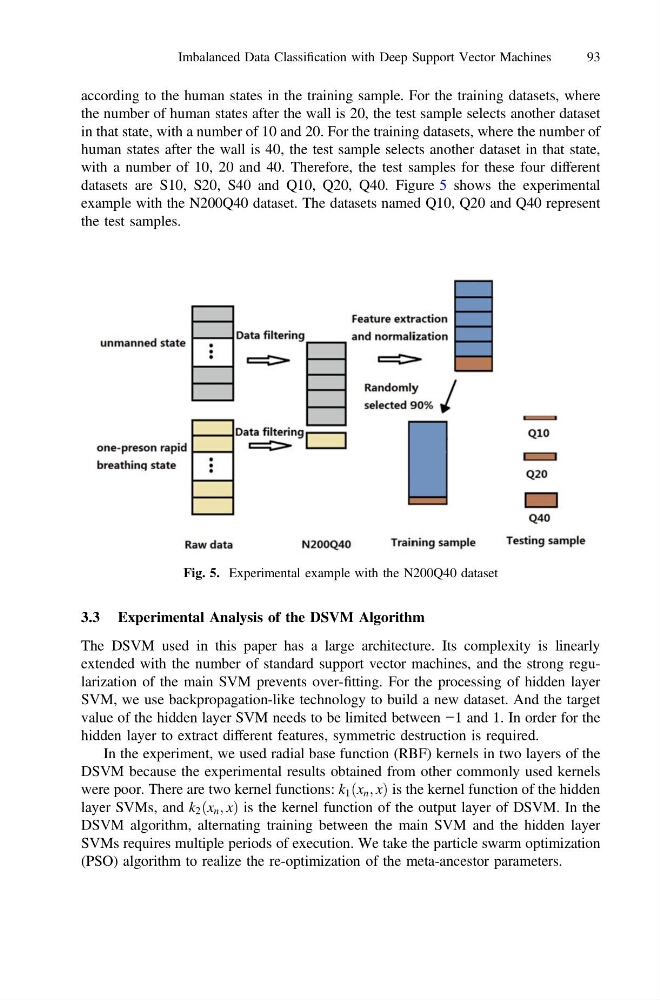
datasets are S10, S20, S40 and Q10, Q20, Q40. Figure 5 shows the experimental
example with the N200Q40 dataset. The datasets named Q10, Q20 and Q40 represent
the test samples.
3.3 Experimental Analysis of the DSVM Algorithm
The DSVM used in this paper has a large architecture. Its complexity is linearly
extended with the number of standard support vector machines, and the strong regularization of the main SVM prevents over-fitting. For the processing of hidden layer
SVM, we use backpropagation-like technology to build a new dataset. And the target
value of the hidden layer SVM needs to be limited between −1 and 1. In order for the
hidden layer to extract different features, symmetric destruction is required.
In the experiment, we used radial base function (RBF) kernels in two layers of the
DSVM because the experimental results obtained from other commonly used kernels
were poor. There are two kernel functions: k 1 x n ; x
ð
Þis the kernel function of the hidden
layer SVMs, and k 2 x n ; x
ð
Þ is the kernel function of the output layer of DSVM. In the
DSVM algorithm, alternating training between the main SVM and the hidden layer
SVMs requires multiple periods of execution. We take the particle swarm optimization
(PSO) algorithm to realize the re-optimization of the meta-ancestor parameters.
Fig. 5. Experimental example with the N200Q40 dataset
Imbalanced Data Classification with Deep Support Vector Machines
93
the number of human states after the wall is 20, the test sample selects another dataset
in that state, with a number of 10 and 20. For the training datasets, where the number of
human states after the wall is 40, the test sample selects another dataset in that state,
with a number of 10, 20 and 40. Therefore, the test samples for these four different
datasets are S10, S20, S40 and Q10, Q20, Q40. Figure 5 shows the experimental
example with the N200Q40 dataset. The datasets named Q10, Q20 and Q40 represent
the test samples.
3.3 Experimental Analysis of the DSVM Algorithm
The DSVM used in this paper has a large architecture. Its complexity is linearly
extended with the number of standard support vector machines, and the strong regularization of the main SVM prevents over-fitting. For the processing of hidden layer
SVM, we use backpropagation-like technology to build a new dataset. And the target
value of the hidden layer SVM needs to be limited between −1 and 1. In order for the
hidden layer to extract different features, symmetric destruction is required.
In the experiment, we used radial base function (RBF) kernels in two layers of the
DSVM because the experimental results obtained from other commonly used kernels
were poor. There are two kernel functions: k 1 x n ; x
ð
Þis the kernel function of the hidden
layer SVMs, and k 2 x n ; x
ð
Þ is the kernel function of the output layer of DSVM. In the
DSVM algorithm, alternating training between the main SVM and the hidden layer
SVMs requires multiple periods of execution. We take the particle swarm optimization
(PSO) algorithm to realize the re-optimization of the meta-ancestor parameters.
Fig. 5. Experimental example with the N200Q40 dataset
Imbalanced Data Classification with Deep Support Vector Machines
93