

23.2 Programs and Computational Aspects
271
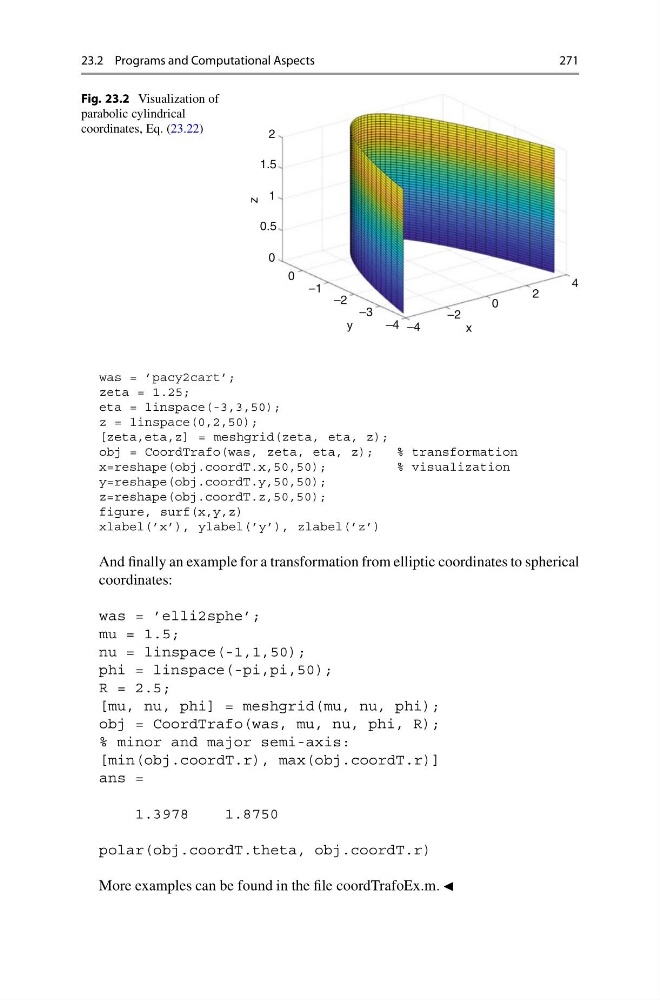
Fig. 23.2 Visualization of
parabolic cylindrical
coordinates, Eq. (23.22)
x
2
1.5
1
0.5
0
0
–1
–2
–3
–4 –4
–2
0
2
4
y
z
was = ’pacy2cart’;
zeta = 1.25;
eta = linspace(-3,3,50);
z = linspace(0,2,50);
[zeta,eta,z] = meshgrid(zeta, eta, z);
obj = CoordTrafo(was, zeta, eta, z);
% transformation
x=reshape(obj.coordT.x,50,50);
% visualization
y=reshape(obj.coordT.y,50,50);
z=reshape(obj.coordT.z,50,50);
figure, surf(x,y,z)
xlabel(’x’), ylabel(’y’), zlabel(’z’)
And finally an example for a transformation from elliptic coordinates to spherical
coordinates:
was = ’elli2sphe’;
mu = 1.5;
nu = linspace(-1,1,50);
phi = linspace(-pi,pi,50);
R = 2.5;
[mu, nu, phi] = meshgrid(mu, nu, phi);
obj = CoordTrafo(was, mu, nu, phi, R);
% minor and major semi-axis:
[min(obj.coordT.r), max(obj.coordT.r)]
ans =
1.3978
1.8750
polar(obj.coordT.theta, obj.coordT.r)
More examples can be found in the file coordTrafoEx.m.
271
Fig. 23.2 Visualization of
parabolic cylindrical
coordinates, Eq. (23.22)
x
2
1.5
1
0.5
0
0
–1
–2
–3
–4 –4
–2
0
2
4
y
z
was = ’pacy2cart’;
zeta = 1.25;
eta = linspace(-3,3,50);
z = linspace(0,2,50);
[zeta,eta,z] = meshgrid(zeta, eta, z);
obj = CoordTrafo(was, zeta, eta, z);
% transformation
x=reshape(obj.coordT.x,50,50);
% visualization
y=reshape(obj.coordT.y,50,50);
z=reshape(obj.coordT.z,50,50);
figure, surf(x,y,z)
xlabel(’x’), ylabel(’y’), zlabel(’z’)
And finally an example for a transformation from elliptic coordinates to spherical
coordinates:
was = ’elli2sphe’;
mu = 1.5;
nu = linspace(-1,1,50);
phi = linspace(-pi,pi,50);
R = 2.5;
[mu, nu, phi] = meshgrid(mu, nu, phi);
obj = CoordTrafo(was, mu, nu, phi, R);
% minor and major semi-axis:
[min(obj.coordT.r), max(obj.coordT.r)]
ans =
1.3978
1.8750
polar(obj.coordT.theta, obj.coordT.r)
More examples can be found in the file coordTrafoEx.m.