

270
23 Coordinate Systems
case transforming from coordinate system A to coordinate system B both coordinate
systems carry a scaling factor, “scal” belongs to system A and “scal2” to system
B. If only one system carries a scaling factor, then “scal2” will be ignored. The
output argument is the class object “obj” with properties “coordIn”, a table with
input coordinates, “coordT”, the table with transformed coordinates, “scal1”, the
first scaling factor, “scal2”, the second scaling factor, and “info” with general
information about scaling and transformation.
Examples
The following code shows the transformation from elliptic cylindrical coordinate
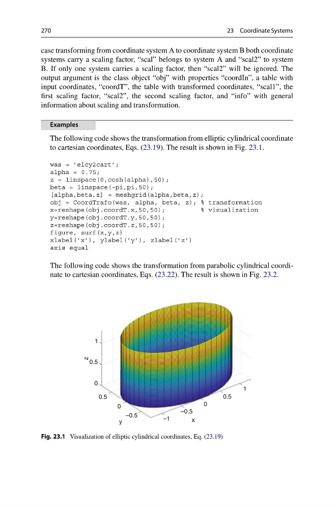
to cartesian coordinates, Eqs. (23.19). The result is shown in Fig. 23.1.
was = ’elcy2cart’;
alpha = 0.75;
z = linspace(0,cosh(alpha),50);
beta = linspace(-pi,pi,50);
[alpha,beta,z] = meshgrid(alpha,beta,z);
obj = CoordTrafo(was, alpha, beta, z); % transformation
x=reshape(obj.coordT.x,50,50);
% visualization
y=reshape(obj.coordT.y,50,50);
z=reshape(obj.coordT.z,50,50);
figure, surf(x,y,z)
xlabel(’x’), ylabel(’y’), zlabel(’z’)
axis equal
The following code shows the transformation from parabolic cylindrical coordinate to cartesian coordinates, Eqs. (23.22). The result is shown in Fig. 23.2.
1
0.5
0
0.5
0
–0.5
–1
–0.5
0
0.5
1
x
y
z
Fig. 23.1 Visualization of elliptic cylindrical coordinates, Eq. (23.19)
23 Coordinate Systems
case transforming from coordinate system A to coordinate system B both coordinate
systems carry a scaling factor, “scal” belongs to system A and “scal2” to system
B. If only one system carries a scaling factor, then “scal2” will be ignored. The
output argument is the class object “obj” with properties “coordIn”, a table with
input coordinates, “coordT”, the table with transformed coordinates, “scal1”, the
first scaling factor, “scal2”, the second scaling factor, and “info” with general
information about scaling and transformation.
Examples
The following code shows the transformation from elliptic cylindrical coordinate
to cartesian coordinates, Eqs. (23.19). The result is shown in Fig. 23.1.
was = ’elcy2cart’;
alpha = 0.75;
z = linspace(0,cosh(alpha),50);
beta = linspace(-pi,pi,50);
[alpha,beta,z] = meshgrid(alpha,beta,z);
obj = CoordTrafo(was, alpha, beta, z); % transformation
x=reshape(obj.coordT.x,50,50);
% visualization
y=reshape(obj.coordT.y,50,50);
z=reshape(obj.coordT.z,50,50);
figure, surf(x,y,z)
xlabel(’x’), ylabel(’y’), zlabel(’z’)
axis equal
The following code shows the transformation from parabolic cylindrical coordinate to cartesian coordinates, Eqs. (23.22). The result is shown in Fig. 23.2.
1
0.5
0
0.5
0
–0.5
–1
–0.5
0
0.5
1
x
y
z
Fig. 23.1 Visualization of elliptic cylindrical coordinates, Eq. (23.19)