

23.1 Separability in Three Dimensions
263
we get
1
r 2
∂
∂r
r
2 ∂
∂r
1
r
nl =
1
r
∂ 2
∂r 2 nl
(23.12b)
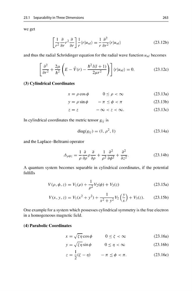
and thus the radial Schrödinger equation for the radial wave function u nl becomes
∂ 2
∂r 2 +
2μ
¯
h 2
E − ˆ
V (r) −
¯
h
2 l(l + 1)
2μr 2
nl = 0.
(23.12c)
(3) Cylindrical Coordinates
x = ρ cos φ
0 ≤ ρ < ∞
(23.13a)
y = ρ sin φ
− π ≤ φ < π
(23.13b)
z = z
− ∞ < z < ∞.
(23.13c)
In cylindrical coordinates the metric tensor g ij is
diag(g ij ) = (1, ρ
2 , 1)
(23.14a)
and the Laplace–Beltrami operator
Δ ρφz =
1
ρ
∂
∂ρ
ρ
∂
∂ρ
+
1
ρ 2
∂ 2
∂φ 2 +
∂ 2
∂z 2 .
(23.14b)
A quantum system becomes separable in cylindrical coordinates, if the potential
fulfills
V (ρ, φ, z) = V 1 (ρ) +
1
ρ 2 V 2 (φ) + V 3 (z)
(23.15a)
V (x, y, z) = V 1 (x
2
+ y
2 ) +
1
x 2 + y 2 V 2
y
x
+ V 3 (z).
(23.15b)
One example for a system which possesses cylindrical symmetry is the free electron
in a homogeneous magnetic field.
(4) Parabolic Coordinates
x =
ζ η cos φ
0 ≤ ζ < ∞
(23.16a)
y =
ζ η sin φ
0 ≤ η < ∞
(23.16b)
z =
1
2
(ζ − η)
− π ≤ φ < π.
(23.16c)
263
we get
1
r 2
∂
∂r
r
2 ∂
∂r
1
r
nl =
1
r
∂ 2
∂r 2 nl
(23.12b)
and thus the radial Schrödinger equation for the radial wave function u nl becomes
∂ 2
∂r 2 +
2μ
¯
h 2
E − ˆ
V (r) −
¯
h
2 l(l + 1)
2μr 2
nl = 0.
(23.12c)
(3) Cylindrical Coordinates
x = ρ cos φ
0 ≤ ρ < ∞
(23.13a)
y = ρ sin φ
− π ≤ φ < π
(23.13b)
z = z
− ∞ < z < ∞.
(23.13c)
In cylindrical coordinates the metric tensor g ij is
diag(g ij ) = (1, ρ
2 , 1)
(23.14a)
and the Laplace–Beltrami operator
Δ ρφz =
1
ρ
∂
∂ρ
ρ
∂
∂ρ
+
1
ρ 2
∂ 2
∂φ 2 +
∂ 2
∂z 2 .
(23.14b)
A quantum system becomes separable in cylindrical coordinates, if the potential
fulfills
V (ρ, φ, z) = V 1 (ρ) +
1
ρ 2 V 2 (φ) + V 3 (z)
(23.15a)
V (x, y, z) = V 1 (x
2
+ y
2 ) +
1
x 2 + y 2 V 2
y
x
+ V 3 (z).
(23.15b)
One example for a system which possesses cylindrical symmetry is the free electron
in a homogeneous magnetic field.
(4) Parabolic Coordinates
x =
ζ η cos φ
0 ≤ ζ < ∞
(23.16a)
y =
ζ η sin φ
0 ≤ η < ∞
(23.16b)
z =
1
2
(ζ − η)
− π ≤ φ < π.
(23.16c)