

264
23 Coordinate Systems
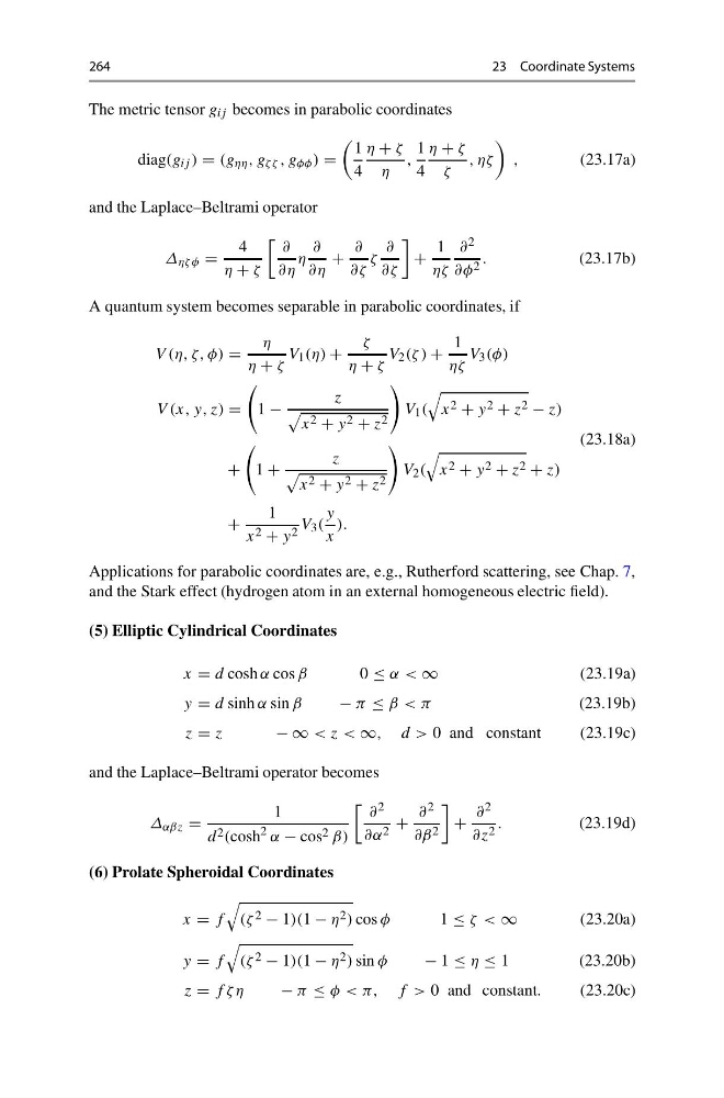
The metric tensor g ij becomes in parabolic coordinates
diag(g ij ) = (g ηη , g ζ ζ , g φφ ) =
1
4
η + ζ
η
,
1
4
η + ζ
ζ
, ηζ
,
(23.17a)
and the Laplace–Beltrami operator
Δ ηζ φ =
4
η + ζ
∂
∂η
η
∂
∂η
+
∂
∂ζ
ζ
∂
∂ζ
+
1
ηζ
∂ 2
∂φ 2 .
(23.17b)
A quantum system becomes separable in parabolic coordinates, if
V (η, ζ, φ) =
η
η + ζ
V 1 (η) +
ζ
η + ζ
V 2 (ζ ) +
1
ηζ
V 3 (φ)
V (x, y, z) =
1 −
z
x 2 + y 2 + z 2
V 1 (
x 2 + y 2 + z 2 − z)
+
1 +
z
x 2 + y 2 + z 2
V 2 (
x 2 + y 2 + z 2 + z)
+
1
x 2 + y 2 V 3 (
y
x
).
(23.18a)
Applications for parabolic coordinates are, e.g., Rutherford scattering, see Chap. 7,
and the Stark effect (hydrogen atom in an external homogeneous electric field).
(5) Elliptic Cylindrical Coordinates
x = d cosh α cos β
0 ≤ α < ∞
(23.19a)
y = d sinh α sin β
− π ≤ β < π
(23.19b)
z = z
− ∞ < z < ∞, d > 0 and constant
(23.19c)
and the Laplace–Beltrami operator becomes
Δ αβz =
1
d 2 (cosh
2 α − cos 2 β)
∂ 2
∂α 2 +
∂ 2
∂β 2
+
∂ 2
∂z 2 .
(23.19d)
(6) Prolate Spheroidal Coordinates
x = f
(ζ 2 − 1)(1 − η 2 ) cos φ
1 ≤ ζ < ∞
(23.20a)
y = f
(ζ 2 − 1)(1 − η 2 ) sin φ
− 1 ≤ η ≤ 1
(23.20b)
z = f ζ η
− π ≤ φ < π, f > 0 and constant.
(23.20c)
23 Coordinate Systems
The metric tensor g ij becomes in parabolic coordinates
diag(g ij ) = (g ηη , g ζ ζ , g φφ ) =
1
4
η + ζ
η
,
1
4
η + ζ
ζ
, ηζ
,
(23.17a)
and the Laplace–Beltrami operator
Δ ηζ φ =
4
η + ζ
∂
∂η
η
∂
∂η
+
∂
∂ζ
ζ
∂
∂ζ
+
1
ηζ
∂ 2
∂φ 2 .
(23.17b)
A quantum system becomes separable in parabolic coordinates, if
V (η, ζ, φ) =
η
η + ζ
V 1 (η) +
ζ
η + ζ
V 2 (ζ ) +
1
ηζ
V 3 (φ)
V (x, y, z) =
1 −
z
x 2 + y 2 + z 2
V 1 (
x 2 + y 2 + z 2 − z)
+
1 +
z
x 2 + y 2 + z 2
V 2 (
x 2 + y 2 + z 2 + z)
+
1
x 2 + y 2 V 3 (
y
x
).
(23.18a)
Applications for parabolic coordinates are, e.g., Rutherford scattering, see Chap. 7,
and the Stark effect (hydrogen atom in an external homogeneous electric field).
(5) Elliptic Cylindrical Coordinates
x = d cosh α cos β
0 ≤ α < ∞
(23.19a)
y = d sinh α sin β
− π ≤ β < π
(23.19b)
z = z
− ∞ < z < ∞, d > 0 and constant
(23.19c)
and the Laplace–Beltrami operator becomes
Δ αβz =
1
d 2 (cosh
2 α − cos 2 β)
∂ 2
∂α 2 +
∂ 2
∂β 2
+
∂ 2
∂z 2 .
(23.19d)
(6) Prolate Spheroidal Coordinates
x = f
(ζ 2 − 1)(1 − η 2 ) cos φ
1 ≤ ζ < ∞
(23.20a)
y = f
(ζ 2 − 1)(1 − η 2 ) sin φ
− 1 ≤ η ≤ 1
(23.20b)
z = f ζ η
− π ≤ φ < π, f > 0 and constant.
(23.20c)