

262
23 Coordinate Systems
V (x, y, z) = V 1 (x
2
+ y
2
+ z
2 ) +
1
x 2 + y 2 + z 2 V 2
x 2 + y 2
z
+
1
x 2 + y 2 V 3
y
x
,
(23.7b)
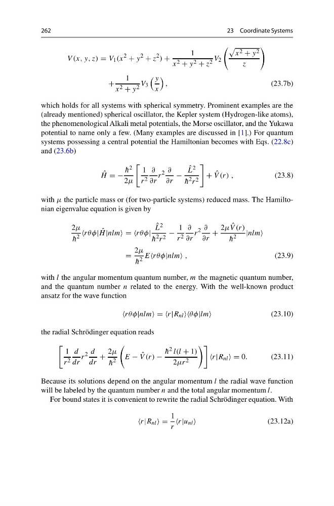
which holds for all systems with spherical symmetry. Prominent examples are the
(already mentioned) spherical oscillator, the Kepler system (Hydrogen-like atoms),
the phenomenological Alkali metal potentials, the Morse oscillator, and the Yukawa
potential to name only a few. (Many examples are discussed in [1].) For quantum
systems possessing a central potential the Hamiltonian becomes with Eqs. (22.8c)
and (23.6b)
ˆ
H = −
¯
h 2
2μ
1
r 2
∂
∂r
r
2 ∂
∂r
−
ˆ
L 2
¯
h 2 r 2
+ ˆ
V (r) ,
(23.8)
with μ the particle mass or (for two-particle systems) reduced mass. The Hamiltonian eigenvalue equation is given by
2μ
¯
h 2 rθφ| ˆ
H |nlm = =rθφ|
ˆ
L 2
¯
h 2 r 2
−
1
r 2
∂
∂r
r
2 ∂
∂r
+
2μ ˆ
V (r)
¯
h 2 |nlm
=
2μ
¯
h 2 Erθφ|nlm ,
(23.9)
with l the angular momentum quantum number, m the magnetic quantum number,
and the quantum number n related to the energy. With the well-known product
ansatz for the wave function
rθφ|nlm = =r|R nl θφ|lm
(23.10)
the radial Schrödinger equation reads
1
r 2
d
dr
r
2 d
dr
+
2μ
¯
h 2
E − ˆ
V (r) −
¯
h 2 l(l + 1)
2μr 2
nl = 0.
(23.11)
Because its solutions depend on the angular momentum l the radial wave function
will be labeled by the quantum number n and the total angular momentum l.
For bound states it is convenient to rewrite the radial Schrödinger equation. With
nl =
1
r
nl
(23.12a)
23 Coordinate Systems
V (x, y, z) = V 1 (x
2
+ y
2
+ z
2 ) +
1
x 2 + y 2 + z 2 V 2
x 2 + y 2
z
+
1
x 2 + y 2 V 3
y
x
,
(23.7b)
which holds for all systems with spherical symmetry. Prominent examples are the
(already mentioned) spherical oscillator, the Kepler system (Hydrogen-like atoms),
the phenomenological Alkali metal potentials, the Morse oscillator, and the Yukawa
potential to name only a few. (Many examples are discussed in [1].) For quantum
systems possessing a central potential the Hamiltonian becomes with Eqs. (22.8c)
and (23.6b)
ˆ
H = −
¯
h 2
2μ
1
r 2
∂
∂r
r
2 ∂
∂r
−
ˆ
L 2
¯
h 2 r 2
+ ˆ
V (r) ,
(23.8)
with μ the particle mass or (for two-particle systems) reduced mass. The Hamiltonian eigenvalue equation is given by
2μ
¯
h 2 rθφ| ˆ
H |nlm = =rθφ|
ˆ
L 2
¯
h 2 r 2
−
1
r 2
∂
∂r
r
2 ∂
∂r
+
2μ ˆ
V (r)
¯
h 2 |nlm
=
2μ
¯
h 2 Erθφ|nlm ,
(23.9)
with l the angular momentum quantum number, m the magnetic quantum number,
and the quantum number n related to the energy. With the well-known product
ansatz for the wave function
rθφ|nlm = =r|R nl θφ|lm
(23.10)
the radial Schrödinger equation reads
1
r 2
d
dr
r
2 d
dr
+
2μ
¯
h 2
E − ˆ
V (r) −
¯
h 2 l(l + 1)
2μr 2
nl = 0.
(23.11)
Because its solutions depend on the angular momentum l the radial wave function
will be labeled by the quantum number n and the total angular momentum l.
For bound states it is convenient to rewrite the radial Schrödinger equation. With
nl =
1
r
nl
(23.12a)