

194
15 Orthogonal Polynomials: General Aspects
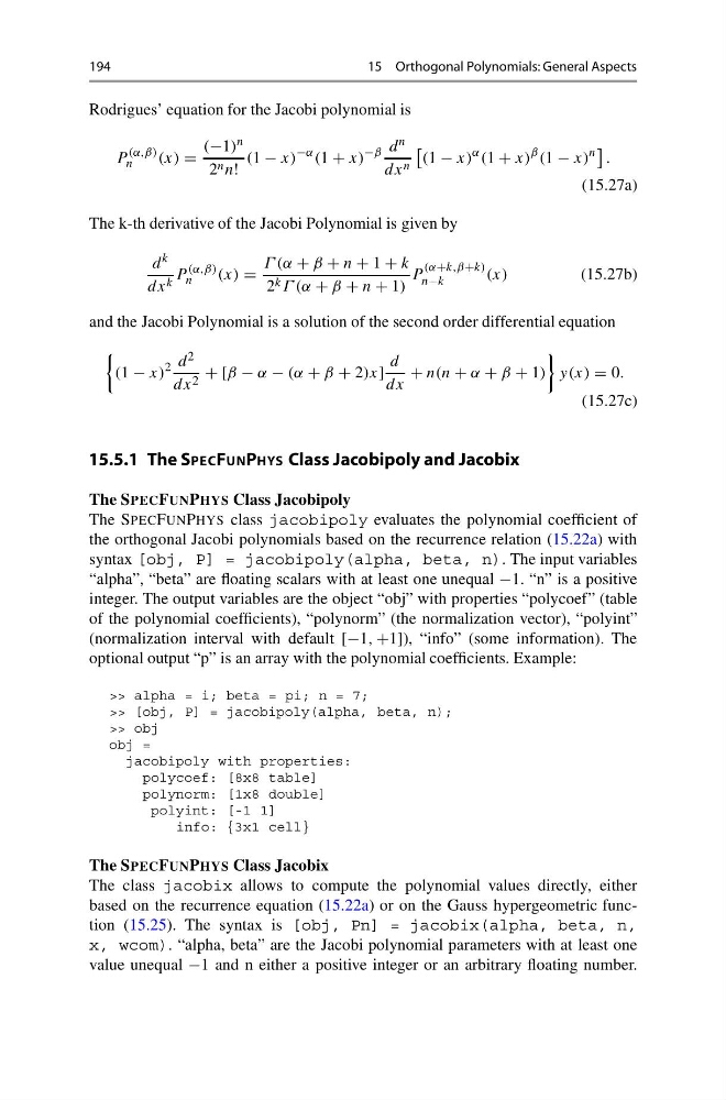
Rodrigues’ equation for the Jacobi polynomial is
P
(α,β)
n
(x) =
(−1) n
2 n n!
(1 − x)
−α (1 + x)
−β d n
dx n
(1 − x)
α (1 + x)
β (1 − x)
n
.
(15.27a)
The k-th derivative of the Jacobi Polynomial is given by
d k
dx k P
(α,β)
n
(x) =
Γ (α + β + n + 1 + k
2 k Γ (α + β + n + 1)
P
(α+k,β+k)
n−k
(x)
(15.27b)
and the Jacobi Polynomial is a solution of the second order differential equation
(1 − x)
2 d 2
dx 2 + [β − α − (α + β + 2)x]
d
dx
+ n(n + α + β + 1)
y(x) = 0.
(15.27c)
15.5.1 The SPECFUNPHYS Class Jacobipoly and Jacobix
The SPECFUNPHYS Class Jacobipoly
The SPECFUNPHYS class jacobipoly evaluates the polynomial coefficient of
the orthogonal Jacobi polynomials based on the recurrence relation (15.22a) with
syntax [obj, P] = jacobipoly(alpha, beta, n). The input variables
“alpha”, “beta” are floating scalars with at least one unequal −1. “n” is a positive
integer. The output variables are the object “obj” with properties “polycoef” (table
of the polynomial coefficients), “polynorm” (the normalization vector), “polyint”
(normalization interval with default [−1, +1]), “info” (some information). The
optional output “p” is an array with the polynomial coefficients. Example:
>> alpha = i; beta = pi; n = 7;
>> [obj, P] = jacobipoly(alpha, beta, n);
>> obj
obj =
jacobipoly with properties:
polycoef: [8x8 table]
polynorm: [1x8 double]
polyint: [-1 1]
info: {3x1 cell}
The SPECFUNPHYS Class Jacobix
The class jacobix allows to compute the polynomial values directly, either
based on the recurrence equation (15.22a) or on the Gauss hypergeometric function (15.25). The syntax is [obj, Pn] = jacobix(alpha, beta, n,
x, wcom). “alpha, beta” are the Jacobi polynomial parameters with at least one
value unequal −1 and n either a positive integer or an arbitrary floating number.
15 Orthogonal Polynomials: General Aspects
Rodrigues’ equation for the Jacobi polynomial is
P
(α,β)
n
(x) =
(−1) n
2 n n!
(1 − x)
−α (1 + x)
−β d n
dx n
(1 − x)
α (1 + x)
β (1 − x)
n
.
(15.27a)
The k-th derivative of the Jacobi Polynomial is given by
d k
dx k P
(α,β)
n
(x) =
Γ (α + β + n + 1 + k
2 k Γ (α + β + n + 1)
P
(α+k,β+k)
n−k
(x)
(15.27b)
and the Jacobi Polynomial is a solution of the second order differential equation
(1 − x)
2 d 2
dx 2 + [β − α − (α + β + 2)x]
d
dx
+ n(n + α + β + 1)
y(x) = 0.
(15.27c)
15.5.1 The SPECFUNPHYS Class Jacobipoly and Jacobix
The SPECFUNPHYS Class Jacobipoly
The SPECFUNPHYS class jacobipoly evaluates the polynomial coefficient of
the orthogonal Jacobi polynomials based on the recurrence relation (15.22a) with
syntax [obj, P] = jacobipoly(alpha, beta, n). The input variables
“alpha”, “beta” are floating scalars with at least one unequal −1. “n” is a positive
integer. The output variables are the object “obj” with properties “polycoef” (table
of the polynomial coefficients), “polynorm” (the normalization vector), “polyint”
(normalization interval with default [−1, +1]), “info” (some information). The
optional output “p” is an array with the polynomial coefficients. Example:
>> alpha = i; beta = pi; n = 7;
>> [obj, P] = jacobipoly(alpha, beta, n);
>> obj
obj =
jacobipoly with properties:
polycoef: [8x8 table]
polynorm: [1x8 double]
polyint: [-1 1]
info: {3x1 cell}
The SPECFUNPHYS Class Jacobix
The class jacobix allows to compute the polynomial values directly, either
based on the recurrence equation (15.22a) or on the Gauss hypergeometric function (15.25). The syntax is [obj, Pn] = jacobix(alpha, beta, n,
x, wcom). “alpha, beta” are the Jacobi polynomial parameters with at least one
value unequal −1 and n either a positive integer or an arbitrary floating number.