

15.5 Jacobi Polynomials
195
In the last case the evaluation is based on the hypergeometric function. This is
also the case if the optional input variable “wcom” has the value “2F1”. In case
the evaluation is based on the recurrence formula all degrees up to the value of
n will be computed. The input variable “x” could be an arbitrary complex array.
The output variables are the object “obj” and an array with the polynomial values
“Pn”. The object “obj” comes with the properties “value” (the polynomial value),
“z” (the position at which the function was evaluated), “degree” (the input variable
n), “alpha” and “beta” (the Jacobi polynomial parameters), and “info” (with some
general information). The class jacobix comes in addition with a plot-method
with syntax (equal the gegenbauerx plot-method) obj = plot(obj, nl),
“obj” an object of the class and “nl” an optional integer vector of the polynomial
degrees which should be plotted. As an application example of the class jacobix
we evaluate the Wigner rotation function.
Example
The Wigner rotation function can be computed via Jacobi polynomials
d
l
m,m (β) =
(l + m)!(l − m)!
(l + m )!(l − m )!
1
2
(cos β/2)
m+m
(sin β/2)
m−m
P
(m−m ,m+m )
l−m
(cos β).
(15.28)
The polynomial coefficients and degree are given by the angular momentum l
and the magnetic quantum numbers m, m by d l
m,m (β) ↔ P
m−m ,m+m
l−m
(cos β).
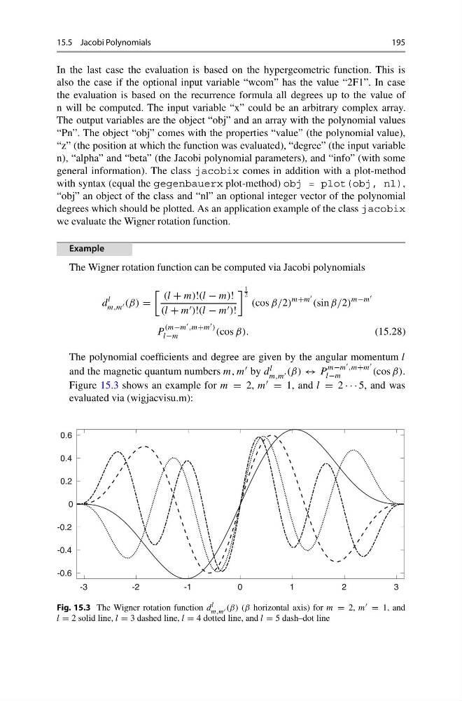
Figure 15.3 shows an example for m = 2, m = 1, and l = 2 · · · 5, and was
evaluated via (wigjacvisu.m):
- 3
- 2
- 1
0
1
2
3
-0.6
-0.4
-0.2
0
0.2
0.4
0.6
Fig. 15.3 The Wigner rotation function d
l
m,m (β) (β horizontal axis) for m = 2, m = 1, and
l = 2 solid line, l = 3 dashed line, l = 4 dotted line, and l = 5 dash–dot line
195
In the last case the evaluation is based on the hypergeometric function. This is
also the case if the optional input variable “wcom” has the value “2F1”. In case
the evaluation is based on the recurrence formula all degrees up to the value of
n will be computed. The input variable “x” could be an arbitrary complex array.
The output variables are the object “obj” and an array with the polynomial values
“Pn”. The object “obj” comes with the properties “value” (the polynomial value),
“z” (the position at which the function was evaluated), “degree” (the input variable
n), “alpha” and “beta” (the Jacobi polynomial parameters), and “info” (with some
general information). The class jacobix comes in addition with a plot-method
with syntax (equal the gegenbauerx plot-method) obj = plot(obj, nl),
“obj” an object of the class and “nl” an optional integer vector of the polynomial
degrees which should be plotted. As an application example of the class jacobix
we evaluate the Wigner rotation function.
Example
The Wigner rotation function can be computed via Jacobi polynomials
d
l
m,m (β) =
(l + m)!(l − m)!
(l + m )!(l − m )!
1
2
(cos β/2)
m+m
(sin β/2)
m−m
P
(m−m ,m+m )
l−m
(cos β).
(15.28)
The polynomial coefficients and degree are given by the angular momentum l
and the magnetic quantum numbers m, m by d l
m,m (β) ↔ P
m−m ,m+m
l−m
(cos β).
Figure 15.3 shows an example for m = 2, m = 1, and l = 2 · · · 5, and was
evaluated via (wigjacvisu.m):
- 3
- 2
- 1
0
1
2
3
-0.6
-0.4
-0.2
0
0.2
0.4
0.6
Fig. 15.3 The Wigner rotation function d
l
m,m (β) (β horizontal axis) for m = 2, m = 1, and
l = 2 solid line, l = 3 dashed line, l = 4 dotted line, and l = 5 dash–dot line