

190
15 Orthogonal Polynomials: General Aspects
15.4.1 The SPECFUNPHYS Class gegenbauerpoly
and gegenbauerx
The Class Gegenbauerpoly
The syntax of the class gegenbauerpoly is [obj, C] = gegenbauerpoly(lambda, n), with “lambda” an arbitrary complex number (strictly speaking Gegenbauer polynomials are only defined for λ > −0.5) and the polynomial
degree “n” a positive integer. The output variables are the object “obj” with
properties “polycoef” (table of the polynomial coefficients), “polynorm” (the
normalization vector), “polyint” (normalization interval with default [−1, +1]),
“info” (some information). The optional output “C” is an array with the polynomial
coefficients. Example:
>> lambda = 0.7; n = 5;
>> [obj, C] = gegenbauerpoly(lambda, n);
>> obj
obj =
gegenbauerpoly with properties:
polycoef: [6x6 table]
polynorm: [0.5231 0.6889 0.7925 0.8715 0.9365 0.9924]
polyint: [-1 1]
info: {2x1 cell}
The Class Gegenbauerx
The class gegenbauerx serves for the direct computation of the polynomial
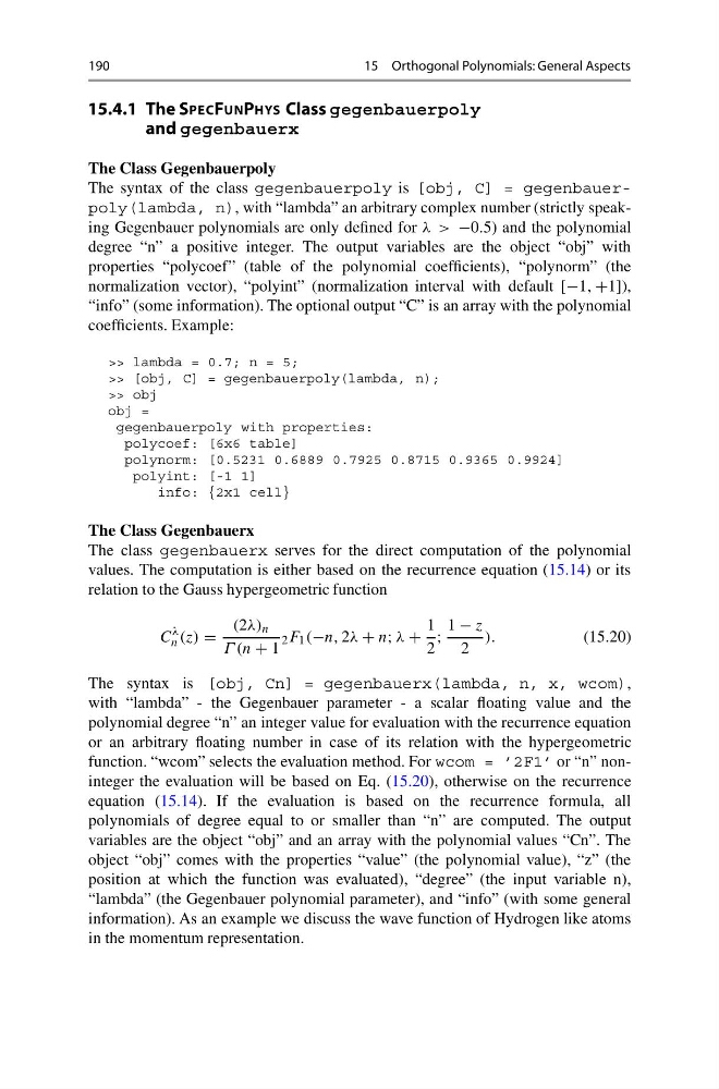
values. The computation is either based on the recurrence equation (15.14) or its
relation to the Gauss hypergeometric function
C
λ
n (z) =
(2λ) n
Γ (n + 1
2 F 1 (−n, 2λ + n; λ +
1
2
;
1 − z
2
).
(15.20)
The syntax is [obj, Cn] = gegenbauerx(lambda, n, x, wcom),
with “lambda” - the Gegenbauer parameter - a scalar floating value and the
polynomial degree “n” an integer value for evaluation with the recurrence equation
or an arbitrary floating number in case of its relation with the hypergeometric
function. “wcom” selects the evaluation method. For wcom = ’2F1’ or “n” noninteger the evaluation will be based on Eq. (15.20), otherwise on the recurrence
equation (15.14). If the evaluation is based on the recurrence formula, all
polynomials of degree equal to or smaller than “n” are computed. The output
variables are the object “obj” and an array with the polynomial values “Cn”. The
object “obj” comes with the properties “value” (the polynomial value), “z” (the
position at which the function was evaluated), “degree” (the input variable n),
“lambda” (the Gegenbauer polynomial parameter), and “info” (with some general
information). As an example we discuss the wave function of Hydrogen like atoms
in the momentum representation.
15 Orthogonal Polynomials: General Aspects
15.4.1 The SPECFUNPHYS Class gegenbauerpoly
and gegenbauerx
The Class Gegenbauerpoly
The syntax of the class gegenbauerpoly is [obj, C] = gegenbauerpoly(lambda, n), with “lambda” an arbitrary complex number (strictly speaking Gegenbauer polynomials are only defined for λ > −0.5) and the polynomial
degree “n” a positive integer. The output variables are the object “obj” with
properties “polycoef” (table of the polynomial coefficients), “polynorm” (the
normalization vector), “polyint” (normalization interval with default [−1, +1]),
“info” (some information). The optional output “C” is an array with the polynomial
coefficients. Example:
>> lambda = 0.7; n = 5;
>> [obj, C] = gegenbauerpoly(lambda, n);
>> obj
obj =
gegenbauerpoly with properties:
polycoef: [6x6 table]
polynorm: [0.5231 0.6889 0.7925 0.8715 0.9365 0.9924]
polyint: [-1 1]
info: {2x1 cell}
The Class Gegenbauerx
The class gegenbauerx serves for the direct computation of the polynomial
values. The computation is either based on the recurrence equation (15.14) or its
relation to the Gauss hypergeometric function
C
λ
n (z) =
(2λ) n
Γ (n + 1
2 F 1 (−n, 2λ + n; λ +
1
2
;
1 − z
2
).
(15.20)
The syntax is [obj, Cn] = gegenbauerx(lambda, n, x, wcom),
with “lambda” - the Gegenbauer parameter - a scalar floating value and the
polynomial degree “n” an integer value for evaluation with the recurrence equation
or an arbitrary floating number in case of its relation with the hypergeometric
function. “wcom” selects the evaluation method. For wcom = ’2F1’ or “n” noninteger the evaluation will be based on Eq. (15.20), otherwise on the recurrence
equation (15.14). If the evaluation is based on the recurrence formula, all
polynomials of degree equal to or smaller than “n” are computed. The output
variables are the object “obj” and an array with the polynomial values “Cn”. The
object “obj” comes with the properties “value” (the polynomial value), “z” (the
position at which the function was evaluated), “degree” (the input variable n),
“lambda” (the Gegenbauer polynomial parameter), and “info” (with some general
information). As an example we discuss the wave function of Hydrogen like atoms
in the momentum representation.