

15.4 Gegenbauer Polynomials
191
0
1
2
3
4
5
6
7
-0.5
0
0.5
1
1.5
P( )
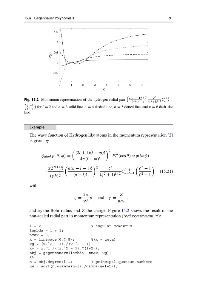
Fig. 15.2 Momentum representation of the hydrogen radial part
n(n−l−1)!
(n+l)!
1
2
ζ l
(ζ 2 +1) l+2 C
l+1
n−l−1
ζ 2 −1
ζ 2 +1
for l = 2 and n = 3 solid line, n = 4 dashed line, n = 5 dotted line, and n = 6 dash–dot
line
Example
The wave function of Hydrogen like atoms in the momentum representation [2]
is given by
φ nlm (p, θ, φ) =
(2l + 1)(l − m)!
4π(l + m)!
1
2
P
m
l (cos θ) exp(imφ)
·
π2 2l+4 l!
(γ h)
3
2
n(n − l − 1)!
(n + l)!
1
2
ζ l
(ζ 2 + 1) l+2 C
l+1
n−l−1
ζ 2 − 1
ζ 2 + 1
(15.21)
with
ζ =
2π
γ h
p and γ =
Z
na o
;
and a 0 the Bohr radius and Z the charge. Figure 15.2 shows the result of the
non-scaled radial part in momentum representation (hydrogenmom.m):
l = 2;
% angular momentum
lambda = l + 1;
nmax = 3;
x = linspace(0,7.5);
%(x = zeta)
xg = (x.^2 - 1)./(x.^2 + 1);
xv = x.^l./((x.^2 + 1).^(l+2));
obj = gegenbauerx(lambda, nmax, xg);
%%
n = obj.degree+l+1;
% principal quantum numbers
ns = sqrt(n. * gamma(n-l)./gamma(n+l+1));
191
0
1
2
3
4
5
6
7
-0.5
0
0.5
1
1.5
P( )
Fig. 15.2 Momentum representation of the hydrogen radial part
n(n−l−1)!
(n+l)!
1
2
ζ l
(ζ 2 +1) l+2 C
l+1
n−l−1
ζ 2 −1
ζ 2 +1
for l = 2 and n = 3 solid line, n = 4 dashed line, n = 5 dotted line, and n = 6 dash–dot
line
Example
The wave function of Hydrogen like atoms in the momentum representation [2]
is given by
φ nlm (p, θ, φ) =
(2l + 1)(l − m)!
4π(l + m)!
1
2
P
m
l (cos θ) exp(imφ)
·
π2 2l+4 l!
(γ h)
3
2
n(n − l − 1)!
(n + l)!
1
2
ζ l
(ζ 2 + 1) l+2 C
l+1
n−l−1
ζ 2 − 1
ζ 2 + 1
(15.21)
with
ζ =
2π
γ h
p and γ =
Z
na o
;
and a 0 the Bohr radius and Z the charge. Figure 15.2 shows the result of the
non-scaled radial part in momentum representation (hydrogenmom.m):
l = 2;
% angular momentum
lambda = l + 1;
nmax = 3;
x = linspace(0,7.5);
%(x = zeta)
xg = (x.^2 - 1)./(x.^2 + 1);
xv = x.^l./((x.^2 + 1).^(l+2));
obj = gegenbauerx(lambda, nmax, xg);
%%
n = obj.degree+l+1;
% principal quantum numbers
ns = sqrt(n. * gamma(n-l)./gamma(n+l+1));