

184
15 Orthogonal Polynomials: General Aspects
+
⎛
⎜
⎜
⎜
⎜
⎜
⎜
⎝
0
0
0
. . .
k N−1
k N
φ N (x)
⎞
⎟
⎟
⎟
⎟
⎟
⎟
⎠
(15.5)
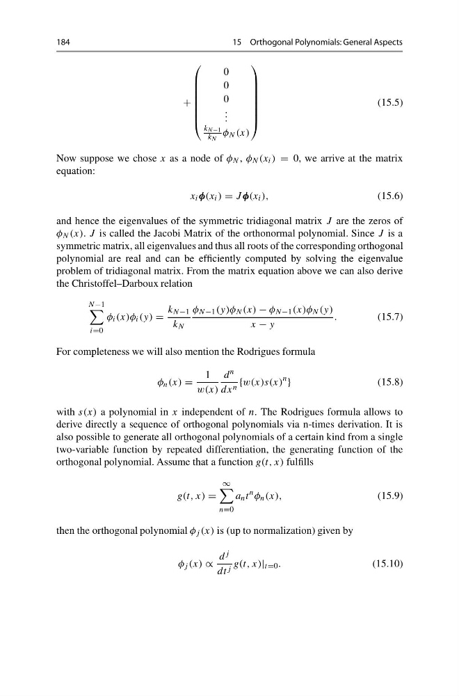
Now suppose we chose x as a node of φ N , φ N (x i ) = 0, we arrive at the matrix
equation:
x i φ(x i ) = J φ(x i ),
(15.6)
and hence the eigenvalues of the symmetric tridiagonal matrix J are the zeros of
φ N (x). J is called the Jacobi Matrix of the orthonormal polynomial. Since J is a
symmetric matrix, all eigenvalues and thus all roots of the corresponding orthogonal
polynomial are real and can be efficiently computed by solving the eigenvalue
problem of tridiagonal matrix. From the matrix equation above we can also derive
the Christoffel–Darboux relation
N−1
i=0
φ i (x)φ i (y) =
k N−1
k N
φ N−1 (y)φ N (x) − φ N−1 (x)φ N (y)
x − y
.
(15.7)
For completeness we will also mention the Rodrigues formula
φ n (x) =
1
w(x)
d n
dx n {w(x)s(x)
n
}
(15.8)
with s(x) a polynomial in x independent of n. The Rodrigues formula allows to
derive directly a sequence of orthogonal polynomials via n-times derivation. It is
also possible to generate all orthogonal polynomials of a certain kind from a single
two-variable function by repeated differentiation, the generating function of the
orthogonal polynomial. Assume that a function g(t, x) fulfills
g(t, x) =
∞
n=0
a n t
n φ n (x),
(15.9)
then the orthogonal polynomial φ j (x) is (up to normalization) given by
φ j (x) ∝
d j
dt j g(t, x)| t =0 .
(15.10)
15 Orthogonal Polynomials: General Aspects
+
⎛
⎜
⎜
⎜
⎜
⎜
⎜
⎝
0
0
0
. . .
k N−1
k N
φ N (x)
⎞
⎟
⎟
⎟
⎟
⎟
⎟
⎠
(15.5)
Now suppose we chose x as a node of φ N , φ N (x i ) = 0, we arrive at the matrix
equation:
x i φ(x i ) = J φ(x i ),
(15.6)
and hence the eigenvalues of the symmetric tridiagonal matrix J are the zeros of
φ N (x). J is called the Jacobi Matrix of the orthonormal polynomial. Since J is a
symmetric matrix, all eigenvalues and thus all roots of the corresponding orthogonal
polynomial are real and can be efficiently computed by solving the eigenvalue
problem of tridiagonal matrix. From the matrix equation above we can also derive
the Christoffel–Darboux relation
N−1
i=0
φ i (x)φ i (y) =
k N−1
k N
φ N−1 (y)φ N (x) − φ N−1 (x)φ N (y)
x − y
.
(15.7)
For completeness we will also mention the Rodrigues formula
φ n (x) =
1
w(x)
d n
dx n {w(x)s(x)
n
}
(15.8)
with s(x) a polynomial in x independent of n. The Rodrigues formula allows to
derive directly a sequence of orthogonal polynomials via n-times derivation. It is
also possible to generate all orthogonal polynomials of a certain kind from a single
two-variable function by repeated differentiation, the generating function of the
orthogonal polynomial. Assume that a function g(t, x) fulfills
g(t, x) =
∞
n=0
a n t
n φ n (x),
(15.9)
then the orthogonal polynomial φ j (x) is (up to normalization) given by
φ j (x) ∝
d j
dt j g(t, x)| t =0 .
(15.10)