

15.3 The Classes orthpoly and polymeth
185
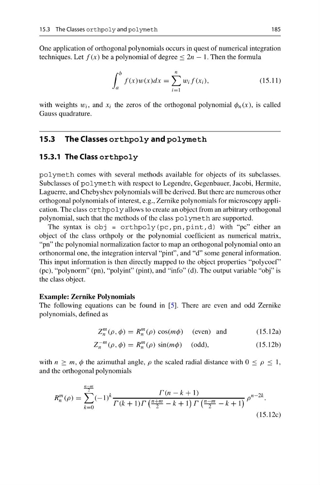
One application of orthogonal polynomials occurs in quest of numerical integration
techniques. Let f (x) be a polynomial of degree ≤ 2n − 1. Then the formula
b
a
f (x)w(x)dx =
n
i=1
w i f (x i ),
(15.11)
with weights w i , and x i the zeros of the orthogonal polynomial φ n (x), is called
Gauss quadrature.
15.3 The Classes orthpoly and polymeth
15.3.1 The Class orthpoly
polymeth comes with several methods available for objects of its subclasses.
Subclasses of polymeth with respect to Legendre, Gegenbauer, Jacobi, Hermite,
Laguerre, and Chebyshev polynomials will be derived. But there are numerous other
orthogonal polynomials of interest, e.g., Zernike polynomials for microscopy application. The class orthpoly allows to create an object from an arbitrary orthogonal
polynomial, such that the methods of the class polymeth are supported.
The syntax is obj = orthpoly(pc,pn,pint,d) with “pc” either an
object of the class orthpoly or the polynomial coefficient as numerical matrix,
“pn” the polynomial normalization factor to map an orthogonal polynomial onto an
orthonormal one, the integration interval “pint”, and “d” some general information.
This input information is then directly mapped to the object properties “polycoef”
(pc), “polynorm” (pn), “polyint” (pint), and “info” (d). The output variable “obj” is
the class object.
Example: Zernike Polynomials
The following equations can be found in [5]. There are even and odd Zernike
polynomials, defined as
Z
m
n (ρ, φ) = R
m
n (ρ) cos(mφ) (even) and
(15.12a)
Z
−m
n (ρ, φ) = R
m
n (ρ) sin(mφ) (odd),
(15.12b)
with n ≥ m, φ the azimuthal angle, ρ the scaled radial distance with 0 ≤ ρ ≤ 1,
and the orthogonal polynomials
R
m
n (ρ) =
n−m
2
k=0
(−1)
k
Γ (n − k + 1)
Γ (k + 1)Γ
n+m
2 − k + 1
Γ
n−m
2 − k + 1
ρ
n−2k .
(15.12c)
185
One application of orthogonal polynomials occurs in quest of numerical integration
techniques. Let f (x) be a polynomial of degree ≤ 2n − 1. Then the formula
b
a
f (x)w(x)dx =
n
i=1
w i f (x i ),
(15.11)
with weights w i , and x i the zeros of the orthogonal polynomial φ n (x), is called
Gauss quadrature.
15.3 The Classes orthpoly and polymeth
15.3.1 The Class orthpoly
polymeth comes with several methods available for objects of its subclasses.
Subclasses of polymeth with respect to Legendre, Gegenbauer, Jacobi, Hermite,
Laguerre, and Chebyshev polynomials will be derived. But there are numerous other
orthogonal polynomials of interest, e.g., Zernike polynomials for microscopy application. The class orthpoly allows to create an object from an arbitrary orthogonal
polynomial, such that the methods of the class polymeth are supported.
The syntax is obj = orthpoly(pc,pn,pint,d) with “pc” either an
object of the class orthpoly or the polynomial coefficient as numerical matrix,
“pn” the polynomial normalization factor to map an orthogonal polynomial onto an
orthonormal one, the integration interval “pint”, and “d” some general information.
This input information is then directly mapped to the object properties “polycoef”
(pc), “polynorm” (pn), “polyint” (pint), and “info” (d). The output variable “obj” is
the class object.
Example: Zernike Polynomials
The following equations can be found in [5]. There are even and odd Zernike
polynomials, defined as
Z
m
n (ρ, φ) = R
m
n (ρ) cos(mφ) (even) and
(15.12a)
Z
−m
n (ρ, φ) = R
m
n (ρ) sin(mφ) (odd),
(15.12b)
with n ≥ m, φ the azimuthal angle, ρ the scaled radial distance with 0 ≤ ρ ≤ 1,
and the orthogonal polynomials
R
m
n (ρ) =
n−m
2
k=0
(−1)
k
Γ (n − k + 1)
Γ (k + 1)Γ
n+m
2 − k + 1
Γ
n−m
2 − k + 1
ρ
n−2k .
(15.12c)