

6 High-Frequency Variability in Neutron-Star Low-Mass X-ray Binaries
289
2 (Hz)
0
200
400
600
800
1000
1200
1 (Hz)
0
200
400
600
800
1000
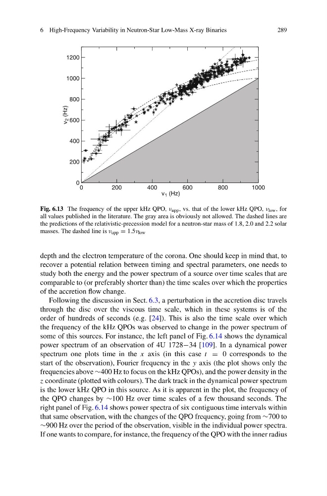
Fig. 6.13 The frequency of the upper kHz QPO, ν upp , vs. that of the lower kHz QPO, ν low , for
all values published in the literature. The gray area is obviously not allowed. The dashed lines are
the predictions of the relativistic-precession model for a neutron-star mass of 1.8, 2.0 and 2.2 solar
masses. The dashed line is ν upp = 1.5ν low
depth and the electron temperature of the corona. One should keep in mind that, to
recover a potential relation between timing and spectral parameters, one needs to
study both the energy and the power spectrum of a source over time scales that are
comparable to (or preferably shorter than) the time scales over which the properties
of the accretion flow change.
Following the discussion in Sect. 6.3, a perturbation in the accretion disc travels
through the disc over the viscous time scale, which in these systems is of the
order of hundreds of seconds (e.g. [24]). This is also the time scale over which
the frequency of the kHz QPOs was observed to change in the power spectrum of
some of this sources. For instance, the left panel of Fig. 6.14 shows the dynamical
power spectrum of an observation of 4U 1728−34 [109]. In a dynamical power
spectrum one plots time in the x axis (in this case t = 0 corresponds to the
start of the observation), Fourier frequency in the y axis (the plot shows only the
frequencies above ∼400 Hz to focus on the kHz QPOs), and the power density in the
z coordinate (plotted with colours). The dark track in the dynamical power spectrum
is the lower kHz QPO in this source. As it is apparent in the plot, the frequency of
the QPO changes by ∼100 Hz over time scales of a few thousand seconds. The
right panel of Fig. 6.14 shows power spectra of six contiguous time intervals within
that same observation, with the changes of the QPO frequency, going from ∼700 to
∼900 Hz over the period of the observation, visible in the individual power spectra.
If one wants to compare, for instance, the frequency of the QPO with the inner radius
289
2 (Hz)
0
200
400
600
800
1000
1200
1 (Hz)
0
200
400
600
800
1000
Fig. 6.13 The frequency of the upper kHz QPO, ν upp , vs. that of the lower kHz QPO, ν low , for
all values published in the literature. The gray area is obviously not allowed. The dashed lines are
the predictions of the relativistic-precession model for a neutron-star mass of 1.8, 2.0 and 2.2 solar
masses. The dashed line is ν upp = 1.5ν low
depth and the electron temperature of the corona. One should keep in mind that, to
recover a potential relation between timing and spectral parameters, one needs to
study both the energy and the power spectrum of a source over time scales that are
comparable to (or preferably shorter than) the time scales over which the properties
of the accretion flow change.
Following the discussion in Sect. 6.3, a perturbation in the accretion disc travels
through the disc over the viscous time scale, which in these systems is of the
order of hundreds of seconds (e.g. [24]). This is also the time scale over which
the frequency of the kHz QPOs was observed to change in the power spectrum of
some of this sources. For instance, the left panel of Fig. 6.14 shows the dynamical
power spectrum of an observation of 4U 1728−34 [109]. In a dynamical power
spectrum one plots time in the x axis (in this case t = 0 corresponds to the
start of the observation), Fourier frequency in the y axis (the plot shows only the
frequencies above ∼400 Hz to focus on the kHz QPOs), and the power density in the
z coordinate (plotted with colours). The dark track in the dynamical power spectrum
is the lower kHz QPO in this source. As it is apparent in the plot, the frequency of
the QPO changes by ∼100 Hz over time scales of a few thousand seconds. The
right panel of Fig. 6.14 shows power spectra of six contiguous time intervals within
that same observation, with the changes of the QPO frequency, going from ∼700 to
∼900 Hz over the period of the observation, visible in the individual power spectra.
If one wants to compare, for instance, the frequency of the QPO with the inner radius