

878
Appendix: All Solutions to the Problems
y
(0) =
y 1 − 0
0.2
, y
(0.2) =
y 2 − y 1
0.2
, y
(0.4) =
y 3 − y 2
0.2
,
y
(0.6) =
y 4 − y 3
0.2
, y
(0.8) =
0 − y 4
0.2
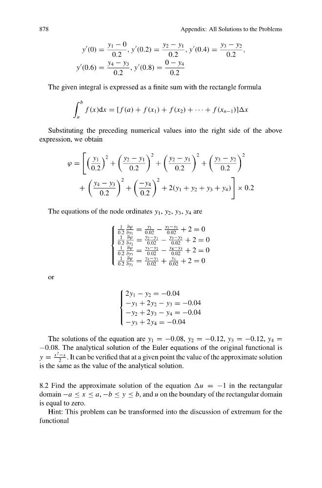
The given integral is expressed as a finite sum with the rectangle formula
b
a
f (x)dx = [ f (a) + f (x 1 ) + f (x 2 ) + · · · + f (x n−1 )]x
Substituting the preceding numerical values into the right side of the above
expression, we obtain
ϕ =
y 1
0.2
2 +
y 2 − y 1
0.2
2
+
y 2 − y 1
0.2
2
+
y 3 − y 2
0.2
2
+
y 4 − y 3
0.2
2
+
−y 4
0.2
2
+ 2(y 1 + y 2 + y 3 + y 4 )
× 0.2
The equations of the node ordinates y 1 , y 2 , y 3 , y 4 are
⎧
⎪ ⎪ ⎪ ⎨
⎪ ⎪ ⎪ ⎩
1
0.2
∂ϕ
∂ y 1
=
y 1
0.02
−
y 2 −y 1
0.02
+ 2 = 0
1
0.2
∂ϕ
∂ y 2
=
y 2 −y 1
0.02
−
y 3 −y 2
0.02
+ 2 = 0
1
0.2
∂ϕ
∂ y 3
=
y 3 −y 2
0.02
−
y 4 −y 3
0.02
+ 2 = 0
1
0.2
∂ϕ
∂ y 1
=
y 4 −y 3
0.02
+
y 4
0.02
+ 2 = 0
or
⎧
⎪ ⎪ ⎨
⎪ ⎪ ⎩
2y 1 − y 2 = −0.04
−y 1 + 2y 2 − y 3 = −0.04
−y 2 + 2y 3 − y 4 = −0.04
−y 3 + 2y 4 = −0.04
The solutions of the equation are y 1 = −0.08, y 2 = −0.12, y 3 = −0.12, y 4 =
−0.08. The analytical solution of the Euler equations of the original functional is
y =
x
2 −x
2
. It can be verified that at a given point the value of the approximate solution
is the same as the value of the analytical solution.
8.2 Find the approximate solution of the equation u = −1 in the rectangular
domain −a ≤ x ≤ a, −b ≤ y ≤ b, and u on the boundary of the rectangular domain
is equal to zero.
Hint: This problem can be transformed into the discussion of extremum for the
functional
Appendix: All Solutions to the Problems
y
(0) =
y 1 − 0
0.2
, y
(0.2) =
y 2 − y 1
0.2
, y
(0.4) =
y 3 − y 2
0.2
,
y
(0.6) =
y 4 − y 3
0.2
, y
(0.8) =
0 − y 4
0.2
The given integral is expressed as a finite sum with the rectangle formula
b
a
f (x)dx = [ f (a) + f (x 1 ) + f (x 2 ) + · · · + f (x n−1 )]x
Substituting the preceding numerical values into the right side of the above
expression, we obtain
ϕ =
y 1
0.2
2 +
y 2 − y 1
0.2
2
+
y 2 − y 1
0.2
2
+
y 3 − y 2
0.2
2
+
y 4 − y 3
0.2
2
+
−y 4
0.2
2
+ 2(y 1 + y 2 + y 3 + y 4 )
× 0.2
The equations of the node ordinates y 1 , y 2 , y 3 , y 4 are
⎧
⎪ ⎪ ⎪ ⎨
⎪ ⎪ ⎪ ⎩
1
0.2
∂ϕ
∂ y 1
=
y 1
0.02
−
y 2 −y 1
0.02
+ 2 = 0
1
0.2
∂ϕ
∂ y 2
=
y 2 −y 1
0.02
−
y 3 −y 2
0.02
+ 2 = 0
1
0.2
∂ϕ
∂ y 3
=
y 3 −y 2
0.02
−
y 4 −y 3
0.02
+ 2 = 0
1
0.2
∂ϕ
∂ y 1
=
y 4 −y 3
0.02
+
y 4
0.02
+ 2 = 0
or
⎧
⎪ ⎪ ⎨
⎪ ⎪ ⎩
2y 1 − y 2 = −0.04
−y 1 + 2y 2 − y 3 = −0.04
−y 2 + 2y 3 − y 4 = −0.04
−y 3 + 2y 4 = −0.04
The solutions of the equation are y 1 = −0.08, y 2 = −0.12, y 3 = −0.12, y 4 =
−0.08. The analytical solution of the Euler equations of the original functional is
y =
x
2 −x
2
. It can be verified that at a given point the value of the approximate solution
is the same as the value of the analytical solution.
8.2 Find the approximate solution of the equation u = −1 in the rectangular
domain −a ≤ x ≤ a, −b ≤ y ≤ b, and u on the boundary of the rectangular domain
is equal to zero.
Hint: This problem can be transformed into the discussion of extremum for the
functional