

Appendix: All Solutions to the Problems
877
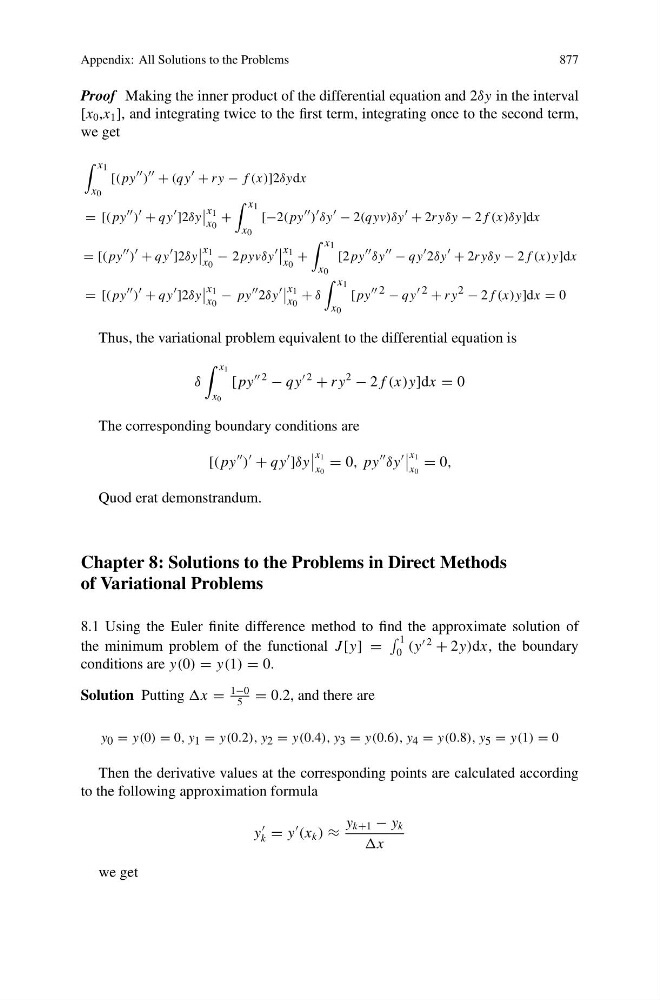
Proof Making the inner product of the differential equation and 2δy in the interval
[x 0 ,x 1 ], and integrating twice to the first term, integrating once to the second term,
we get
x 1
x 0
[( py ) + (qy + r y − f (x)]2δydx
= [( py ) + qy ]2δy
x 1
x 0
+
x 1
x 0
[−2( py ) δy − 2(qyv)δy + 2r yδy − 2 f (x)δy]dx
= [( py ) + qy ]2δy
x 1
x 0
− 2 pyvδy
x 1
x 0
+
x 1
x 0
[2 py δy − qy 2δy + 2r yδy − 2 f (x)y]dx
= [( py ) + qy ]2δy
x 1
x 0
− py 2δy
x 1
x 0
+ δ
x 1
x 0
[ py 2 − qy 2 + r y 2 − 2 f (x)y]dx = 0
Thus, the variational problem equivalent to the differential equation is
δ
x 1
x 0
[ py
2
− qy
2
+ r y
2
− 2 f (x)y]dx = 0
The corresponding boundary conditions are
[( py
)
+ qy
]δy
x 1
x 0
= 0, py
δy
x 1
x 0
= 0,
Quod erat demonstrandum.
Chapter 8: Solutions to the Problems in Direct Methods
of Variational Problems
8.1 Using the Euler finite difference method to find the approximate solution of
the minimum problem of the functional J [y] =
1
0 (y
2
+ 2y)dx, the boundary
conditions are y(0) = y(1) = 0.
Solution Putting x =
1−0
5
= 0.2, and there are
y 0 = y(0) = 0, y 1 = y(0.2), y 2 = y(0.4), y 3 = y(0.6), y 4 = y(0.8), y 5 = y(1) = 0
Then the derivative values at the corresponding points are calculated according
to the following approximation formula
y
k = y
(x k ) ≈
y k+1 − y k
x
we get
877
Proof Making the inner product of the differential equation and 2δy in the interval
[x 0 ,x 1 ], and integrating twice to the first term, integrating once to the second term,
we get
x 1
x 0
[( py ) + (qy + r y − f (x)]2δydx
= [( py ) + qy ]2δy
x 1
x 0
+
x 1
x 0
[−2( py ) δy − 2(qyv)δy + 2r yδy − 2 f (x)δy]dx
= [( py ) + qy ]2δy
x 1
x 0
− 2 pyvδy
x 1
x 0
+
x 1
x 0
[2 py δy − qy 2δy + 2r yδy − 2 f (x)y]dx
= [( py ) + qy ]2δy
x 1
x 0
− py 2δy
x 1
x 0
+ δ
x 1
x 0
[ py 2 − qy 2 + r y 2 − 2 f (x)y]dx = 0
Thus, the variational problem equivalent to the differential equation is
δ
x 1
x 0
[ py
2
− qy
2
+ r y
2
− 2 f (x)y]dx = 0
The corresponding boundary conditions are
[( py
)
+ qy
]δy
x 1
x 0
= 0, py
δy
x 1
x 0
= 0,
Quod erat demonstrandum.
Chapter 8: Solutions to the Problems in Direct Methods
of Variational Problems
8.1 Using the Euler finite difference method to find the approximate solution of
the minimum problem of the functional J [y] =
1
0 (y
2
+ 2y)dx, the boundary
conditions are y(0) = y(1) = 0.
Solution Putting x =
1−0
5
= 0.2, and there are
y 0 = y(0) = 0, y 1 = y(0.2), y 2 = y(0.4), y 3 = y(0.6), y 4 = y(0.8), y 5 = y(1) = 0
Then the derivative values at the corresponding points are calculated according
to the following approximation formula
y
k = y
(x k ) ≈
y k+1 − y k
x
we get